Applied Mathematics
Vol. 4 No. 8 (2013) , Article ID: 35327 , 9 pages DOI:10.4236/am.2013.48154
Optimal System and Invariant Solutions on 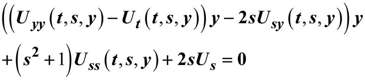
1Department of Mathematics, Faculty of Science, Naresuan University, Phitsanulok, Thailand
2Centre of Excellence in Mathematics, CHE, Bangkok, Thailand
Email: kuntimak@nu.ac.th
Copyright © 2013 Sopita Khamrod. This is an open access article distributed under the Creative Commons Attribution License, which permits unrestricted use, distribution, and reproduction in any medium, provided the original work is properly cited.
Received May 29, 2013; revised June 29, 2013; accepted July 8, 2013
Keywords: Optimal System; Invariant Solutions; Partially Invariant Solutions; Navier-Stokes Equations
ABSTRACT
The purpose of this paper is to find the invariant solutions of the reduction of the Navier-Stokes equations
 where
where  This equation is constructed from the Navier-Stokes equations rising to a partially invariant solutions of the Navier-Stokes equations. Group classification of the admitted Lie algebras of this equation is obtained. Two-dimensional optimal system is constructed from classification of their subalgebras. All invariant solutions corresponding to these subalgebras are presented.
1. Introduction
An invariant solution of a differential equation is a solution of the differential equation which is also an invariant surface of a group admitted by the differential equation. Invariant solution can be found by solving an algebraic equation derived from the given differential equation and the infinitesimals of an admitted Lie group of transformations. Constructing of invariant solutions consists of some steps: choosing a subgroup of the admitted group, finding a representation of solution, substituting the representation into the studied system of equations and the study of compatibility of the obtained (reduced) system of equations.
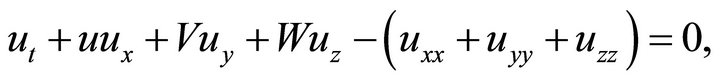
This paper is devoted to use the basic Lie symmetry method for finding the admitted Lie group of the reducetion of the Navier-Stokes equations,
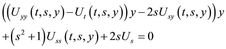 (1)
(1)
where  is a dependent variable and
  are independent variables. This equation is constructed from the Navier-Stokes equations. Subgroups for studying are taken from the part of optimal system of subalgebras considered for the gas dynamics equations [1]. The proposed research will deal with two-dimensional optimal system of subalgebras for the reduction of the Navier-Stokes Equations (1). It is determined for symmetry algebras obtained through classification of their subalgebras. All invariant solutions are presented. They can return to new solutions of the Navier-Stokes equations.
2. Invariant and Partially Invariant Solutions
One of the main goals of application of group analysis to differential equation is construction of representations of solutions. Solutions whose representations are obtained with the help of the admitted group are called invariant or partially invariant solutions. The notion of invariant solution was introduced by Sophus Lie [2]. The notion of a partially invariant solution was introduced by Ovsiannikov [3]. This notion of partially invariant solutions generalizes the notion of an invariant solution, and extends the scope of applications of group analysis for constructing exact solutions of partial differential equations. The algorithm of finding invariant and partially invariant solutions consists of the following steps.
Let  be a Lie algebra with the basis
 . The universal invariant
 ![]() consists of
consists of  functionally independent invariants
where ![]() are the numbers of independent and dependent variables, respectively and
are the numbers of independent and dependent variables, respectively and ![]() is the total rank of the matrix composed by the coefficients of the generators
is the total rank of the matrix composed by the coefficients of the generators . If the rank of the Jacobi matrix
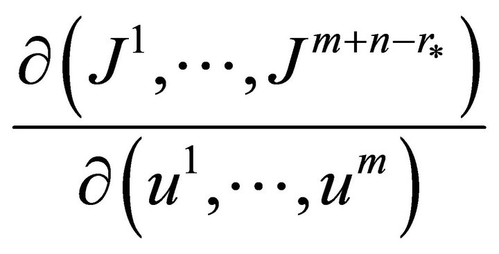
is equal to , then one can choose the first
  invariants
  such that the rank of the Jacobi matrix

is equal to . A partially invariant solution is characterized by two integers:
  and
and . These solutions are also called
  solutions. The number
 ![]() is called the rank of a partially invariant solution. This number gives the number of the independent variables in the representation of the partially invariant solution. The number
is called the rank of a partially invariant solution. This number gives the number of the independent variables in the representation of the partially invariant solution. The number ![]() is called the defect of a partially invariant solution. The defect is the number of the dependent functions which can not be found from the representation of partially invariant solution. The rank
is called the defect of a partially invariant solution. The defect is the number of the dependent functions which can not be found from the representation of partially invariant solution. The rank ![]() and the defect
and the defect ![]() must satisfy the conditions
must satisfy the conditions

where  is the maximum number of invariants which depends on the independent variables only. Note that for invariant solutions,
  and
and .
.
For constructing a representation of a  solution one needs to choose
  invariants and separate the universal invariant in two parts:
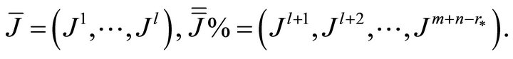
The number  satisfies the inequality
 . The representation of the
  solution is obtained by assuming that the first
  coordinates
  of the universal invariant are functions of the invariants
 :
:
 (2)
(2)
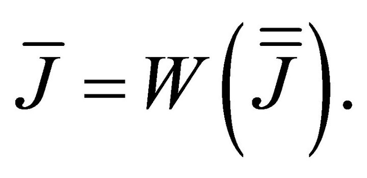
Equation (2) form the invariant part of the representation of a solution. The next assumption about a partially invariant solution is that Equation (2) can be solved for the first  dependent functions, for example,
 (3)
(3)
It is important to note that the functions  are involved in the expressions for the functions
 . The functions
  are called superfluous. The rank and the defect of the
  solution are
 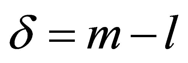 and
and 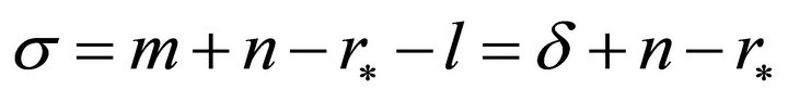 , respectively.
Note that if , the above algorithm is the algorithm for finding a representation of an invariant solution. If
 , then Equation (3) do not define all dependent functions. Since a partially invariant solution satisfies the restrictions (2), this algorithm cuts out some particular solutions from the set of all solutions.
After constructing the representation of an invariant or partially invariant solution (3), it has to be substituted into the original system of equations. The system of equations obtained for the functions  and superfluous functions
  is called the reduced system. This system is overdetermined and requires an analysis of compatibility. Compatibility analysis for invariant solutions is easier than for partially invariant solutions. Another case of partially invariant solutions which is easier than the general case occurs when
  only depends on the independent variables

In this case, a partially invariant solution is called regular, otherwise it is irregular. The number  is called the measure of irregularity.
The process of studying compatibility consists of reducing the overdetermined system of partial differential equations to an involutive system. During this process different subclasses of  partially invariant solutions can be obtained. Some of these subclasses can be
  solutions with subalgebra
 . In this case
 . The study of compatibility of partially invariant solutions with the same rank
 , but with smaller defect
  is simpler than the study of compatibility for
  solutions. In many applications, there is a reduction of a
  solution to a
  solution. In this case the
  solution is called reducible to an invariant solution. The problem of reduction to an invariant solution is important since invariant solutions are usually studied first.
3. The Reduction of the Navier-Stokes Equations
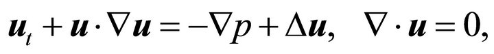
The reduction of the Navier-Stokes equations to partial differential equation in three independent variables is described. Unsteady motion of incompressible viscous fluid is governed by the Navier-Stokes equations
 (4)
(4)
where  is the velocity field,
 ![]() is the fluid pressure,
is the fluid pressure,  is the gradient operator in the three-dimensional space
  and
and ![]() is the Laplacian. A group classification of the Navier-Stokes equations in the three-dimensional case was done in [4]. The Lie group admitted by the Navier-Stokes equations is infinite. Its Lie algebra can be presented in the form of the direct sum
is the Laplacian. A group classification of the Navier-Stokes equations in the three-dimensional case was done in [4]. The Lie group admitted by the Navier-Stokes equations is infinite. Its Lie algebra can be presented in the form of the direct sum , where the infinite-dimensional ideal
  is generated by the operators

with arbitrary functions  and
and . The subalgebra
  has the following basis:
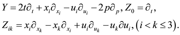
The Galilean algebra  is contained in
 . Several articles [5-11] are devoted to invariant solutions of the Navier-Stokes equations. While partially invariant solutions of the Navier-Stokes equations have been less studied, there has been substantial progress in studying such classes of solutions of inviscid gas dynamics equations [12-19].
In this section analysis of compatibility of regular partially invariant solutions with defect  and rank
  of the subalgebras
  is given. Note that the generator
  is not admitted by the Navier-Stokes equations. The groups are taken from the optimal system constructed for the gas dynamics equations [20].
The Navier-Stokes equations are used in the component form:
 (5)
(5)
 (6)
(6)
 (7)
(7)
 (8)
(8)
The dependent variables  and
and ![]() are functions of the space variables
are functions of the space variables  and time
Invariants of the Lie group corresponding to subalgebra generated by  are
are

The representation of the regular partially invariant solution is
 (9)
(9)
where . For the function
 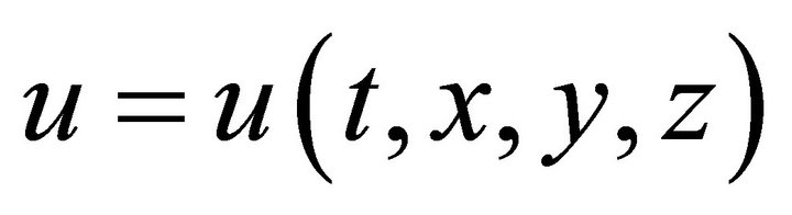 there is no restrictions. Substituting the representation of partially invariant solution (9) into the Navier-Stokes Equations (5)-(8), we obtain
 (10)
(10)
 (11)
(11)
 (12)
(12)
 (13)
(13)
Since  and
and  only depend on
![]() , Equations (11) and (12) can be split with respect to
, Equations (11) and (12) can be split with respect to![]() :
:
 (14)
(14)
 (15)
(15)
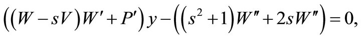
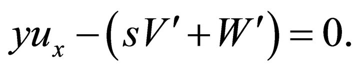
Solving Equations (15), we have

Multiplying the first equation by ![]() and combining it with the second Equation of (14), we obtain
and combining it with the second Equation of (14), we obtain
Let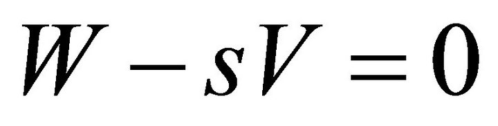 , then
 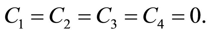 This means that
  and hence
 . Substituting
  and
and  in Equation (13), we have
 . It means that
 ![]() depend on
depend on  or
or  Equation (10) becomes
 (16)
(16)
Thus, there is a solution of the Navier-Stokes equations of the type

where the function  satisfies Equation (16).
If , then
  In this case
 . Note that the Galilei transformation applied to
  and
and , also change
![]() . Substituting
. Substituting  and
and  in Equation (13), we have
  or
or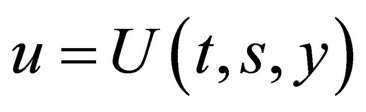 . Equation (10) becomes
 (17)
(17)
Thus, there is a solution of the Navier-Stokes equations of the type

where the function  satisfies Equation (17).
These solutions are partially invariant solution with respect to the group which are not admitted Lie algebra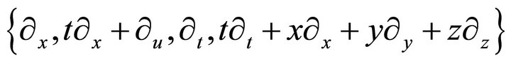 .
.
4. Admitted Group of Equation (16)
In this section, the Lie group admitted by Equation (16) is studied. It was obtained from the Navier-Stokes equations and gives rise to a partially invariant solutions of the Navier-Stokes equations
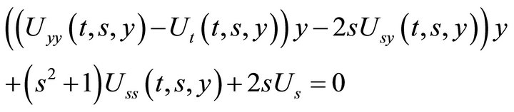
where the function  depends on
  and
and .
.
Assume that the generator has a representation of the form
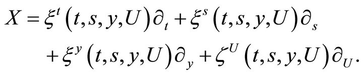
The second prolongation of the operator X is
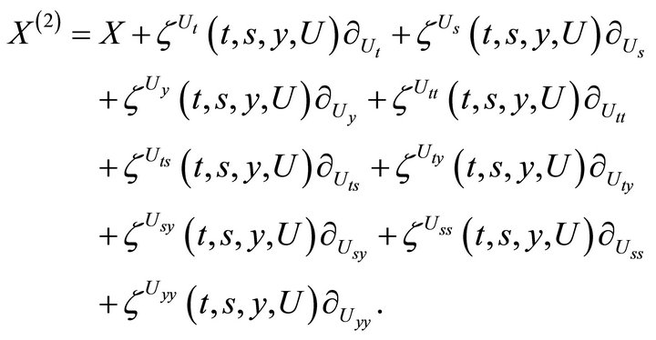
The coefficients of the prolonged operator are defined by formulae
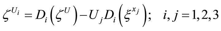
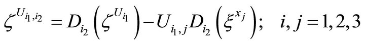
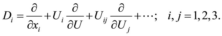
Here we used the notations 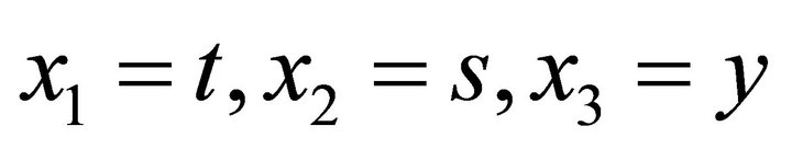 and for the derivatives

The determining equations are
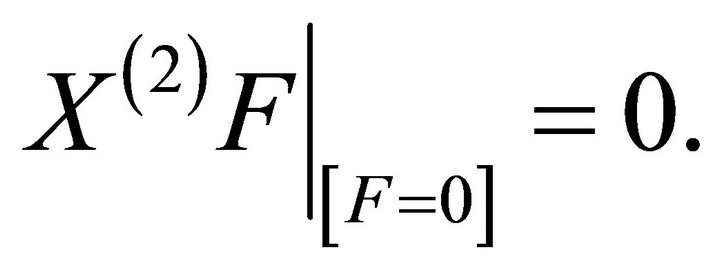 (18)
(18)
All necessary calculations here were carried out on a computer using the symbolic manipulation program REDUCE.
The result of the calculations is the admitted Lie group with the basis of the generators:
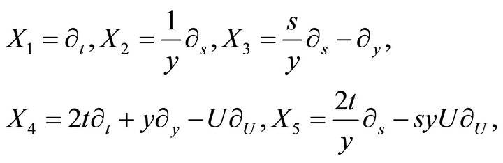 (19)
(19)
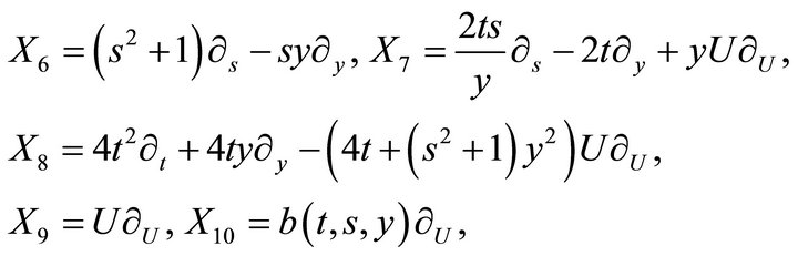
where  is an arbitrary solution of

5. Optimal System of Subalgebras
To obtain all different invariant solutions, we make recourse to the concept of optimal system of subalgebras. This concept follows from the fact that, given a Lie algebra ![]() of order
of order  with
with  the corresponding group of transformations, if two subalgebras of
 ![]() are similar, i.e., they are connected with each other by a transformation of
are similar, i.e., they are connected with each other by a transformation of , then their corresponding invariant solutions are connected with each other by the same transformation. Therefore, in order to construct all the non similar
 ![]() -dimensional subalgebras of
-dimensional subalgebras of![]() , it is sufficient to put into one class all similar subalgebras of a given dimension, say
, it is sufficient to put into one class all similar subalgebras of a given dimension, say![]() , and select a representative from each class. The set of all representatives of these classes is called optimal system of
, and select a representative from each class. The set of all representatives of these classes is called optimal system of ![]() -dimensional subalgebras of
-dimensional subalgebras of![]() . The classification of subalgebras can be done relatively easy for small dimensions. The problem of finding the optimal system is the same as the problem of classifying the orbits of the adjoint transformations. Two-dimensional subalgebras of the optimal system of the Lie algebra spanned by the generators
. The classification of subalgebras can be done relatively easy for small dimensions. The problem of finding the optimal system is the same as the problem of classifying the orbits of the adjoint transformations. Two-dimensional subalgebras of the optimal system of the Lie algebra spanned by the generators  are constructed in [21].
The list of two-dimensional subalgebras of the optimal system of the algebra  is presented in the Table 1, where
  and
and  are arbitrary constants.
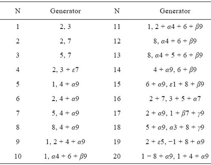
Table 1. Two-dimensional subalgebras of the optimal system of the algebra L9.
6. Invariant Solutions of the Equation (1)
One of the advantages of the symmetry analysis is the possibility to find solutions of the original differential equation by solving reduced equations. The reduced equations are obtained by introducing suitable new variables, determined as invariant functions with respect to the infinitesimal generators. Constructing of invariant solutions consists of some steps: choosing a subgroup of the admitted group, finding a representation of solution, substituting the representation into the studied system of equations and the study of compatibility of the obtained (reduced) system of equations.
Invariant solutions of the Equation (1) are presented in this section. Analysis of invariant solutions is presented in details for four examples.
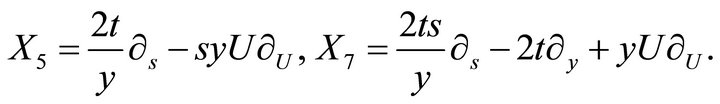
6.1. Subalgebra 3: {5, 7}
The basis of this subalgebra is
In order to find an invariant solution, one needs to find a universal invariant of this subalgebra. Let a function
be an invariant of the generator . This means that
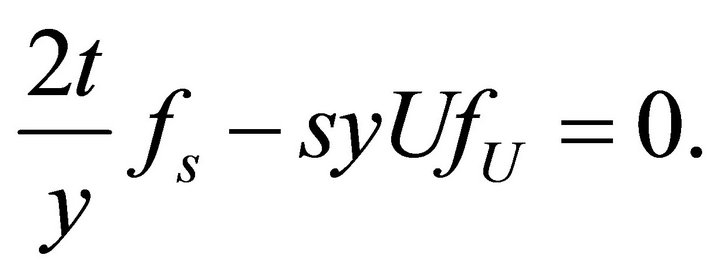
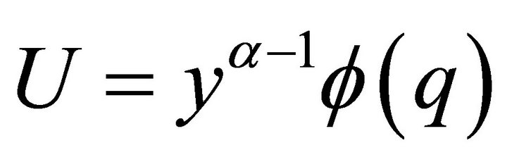
The general solution of this equation is

After substituting it into the equation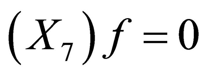 , one obtains the equation
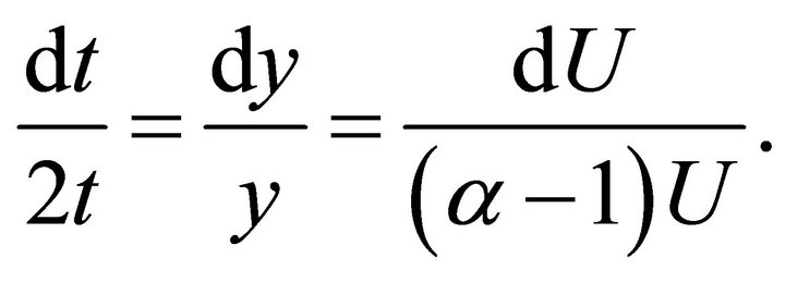
The characteristic system of the last equation is
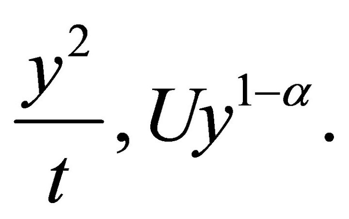
Thus, the universal invariant of this subalgebras consists of invariants

Hence, a representation of the invariant solution is
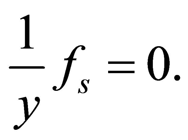
with arbitrary functions . After substituting this representation into Equation (1), one obtains the ordinary differential equation
The general solution of the last equation is
where  is arbitrary constants.
Therefore the invariant solution of the reduction of the Navier-Stokes Equations (1) is
where  is arbitrary constants.
6.2. Subalgebra 6: {2, 4 + α9}
The basis of this subalgebra is

Let a function

be an invariant of the generator . This means that
It means that function  is not depend on
![]() .
.
The general solution of this equation is

After substituting it into the equation 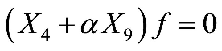 , one obtains the equation
The characteristic system of the last equation is
Thus, the universal invariant of this subalgebras consists of invariants
Hence, a representation of the invariant solution is
with arbitrary functions 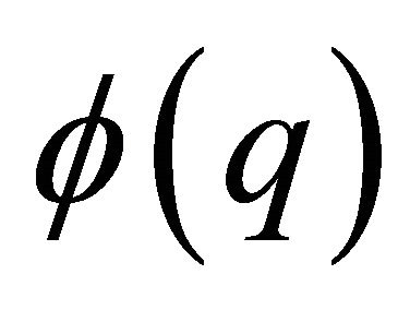 and
and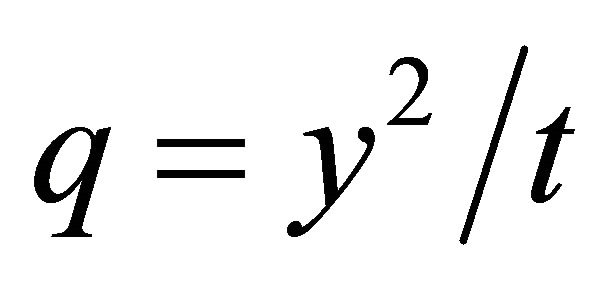 . After substituting this representation into Equation (1), one obtains the ordinary differential equation
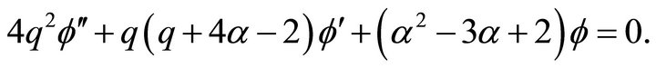
The general solution of the last equation is
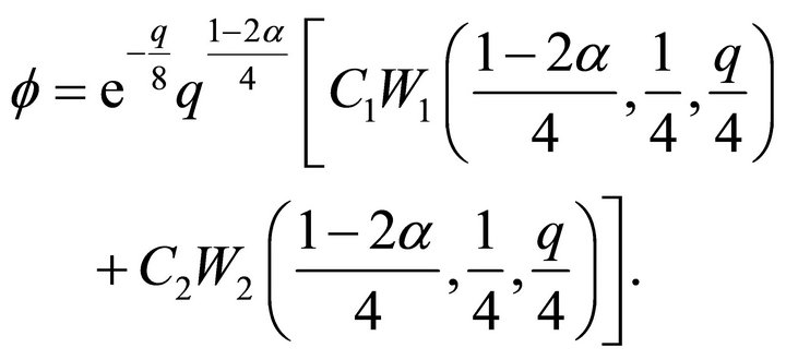
Therefore, the invariant solution of the reduction of the Navier-Stokes Equations (1) is
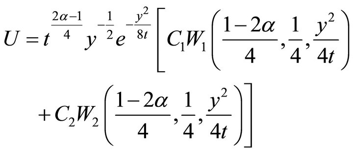
where

are Whittaker functions and  are arbitrary constants.
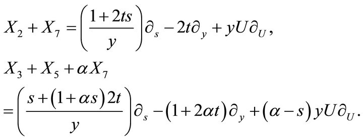
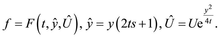
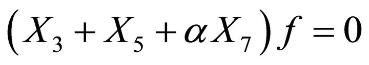
6.3. Subalgebra 16: {2 + 7, 3 + 5 + α7}
The basis of this subalgebra consists of the generators
Let a function

be an invariant of the generator . This means that

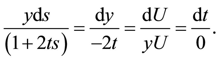
The characteristic system of the last equation is
The general solution of this equation is
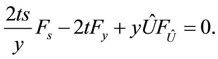
After substituting it into the equation
one obtains the equation
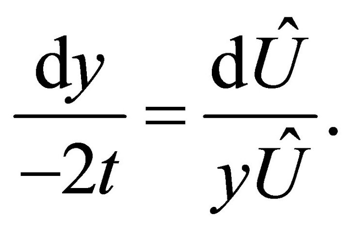
The characteristic system of this equation is
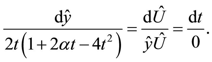
Hence, the universal invariant of this subalgebras consists of invariants
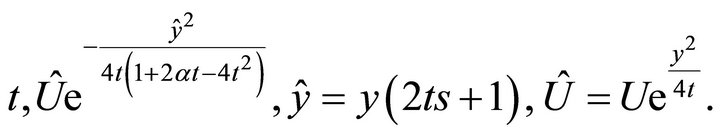
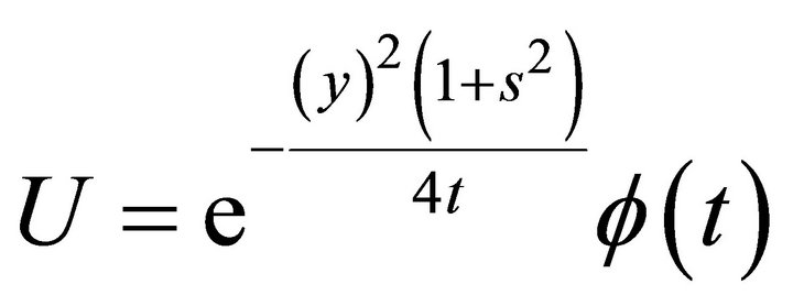
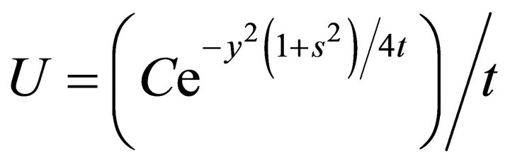
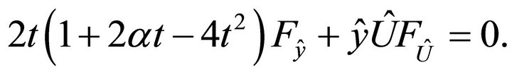
A representation of the invariant solution of this subalgebra has the following form
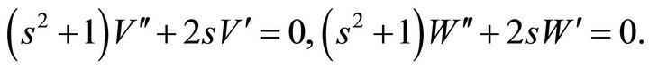
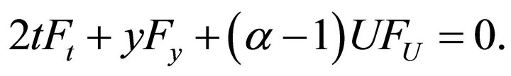
with an arbitrary function . After substituting the representation of the invariant solution into Equation (1), the functions
  has to satisfy the equation
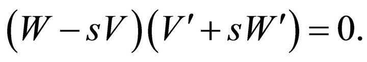

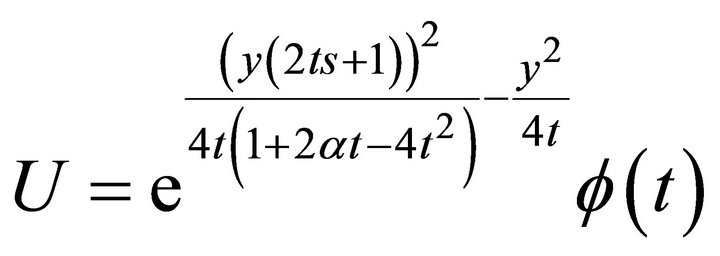
The general solution of the last equation is

where  is constant.
Therefore the invariant solution of the reduction of the Navier-Stokes Equations (1) is
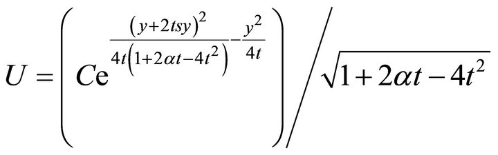
where  is constant.
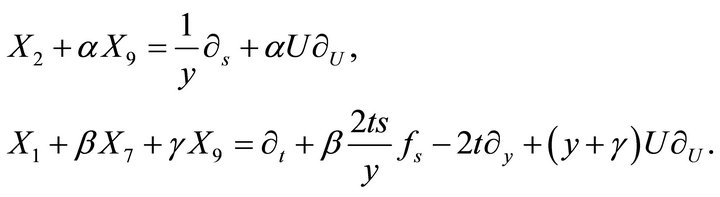
6.4. Subalgebra 17: {2 + α9, 1 + (7 + (9}
The basis of this subalgebra is
Let a function
be an invariant of the generator . This means that

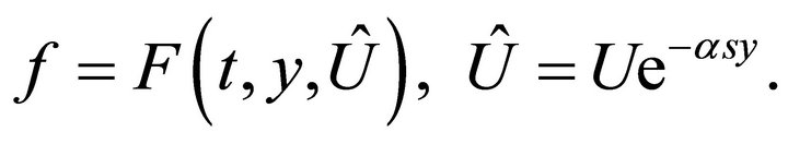
The general solution of this equation is
After substituting it into the equation
one obtains the equation

Thus the universal invariant of this subalgebras consists of invariants
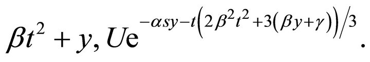
Hence, a representation of the invariant solution is
with arbitrary functions  and
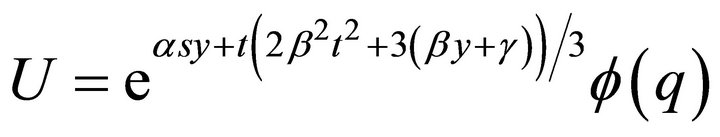
and . After substituting this representation into Equation (1), one obtains the ordinary differential equation

The general solution of the last equation is

Therefore, the invariant solution of the reduction of the Navier-Stokes Equations (1) is
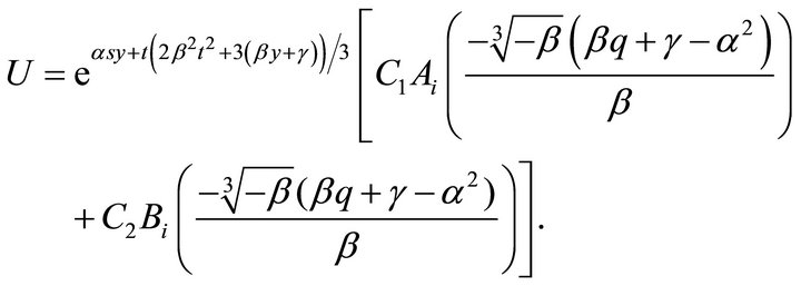
where
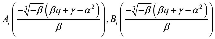
are Airy wave functions and  are arbitrary constants.
The four examples showed that there are solutions of the Navier-Stokes equations, which are partially invariant with respect to not admitted Lie algebra  . They can return to new solutions of the Navier-Stokes equations.
The result of the study of invariant solutions of Equation (1) corresponding to the subalgebras of Table 1 are presented in Table 2.
7. Conclusion
The admitted algebra of the reduction of the NavierStokes Equations (1) is spanned by the generators (19). The optimal systems of two-dimensional subalgebras of the Lie algebra spanned by generators  are obtained: there are 20 classes that have invariant solutions. All invariant solutions corresponding to the optimal system are presented in Table 2. Examples given in the manuscript show that this algorithm can be applied to groups, which are not admitted. These possibilities extend an area of using group analysis for constructing exact solutions.

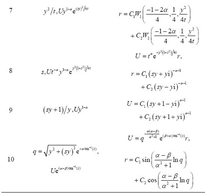
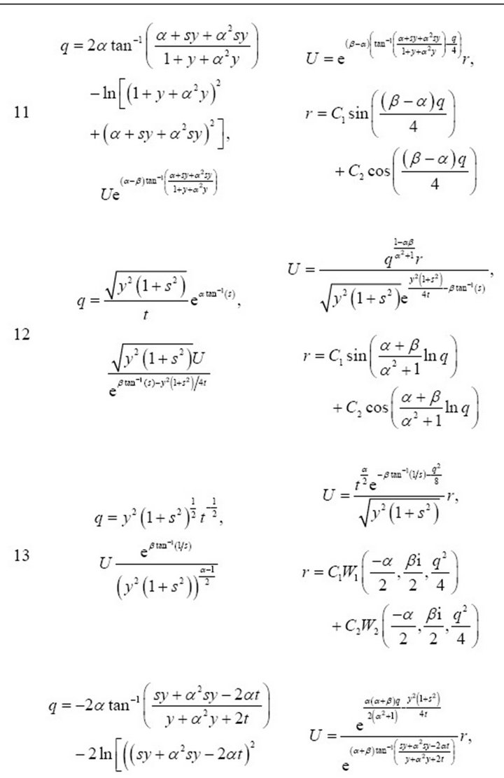
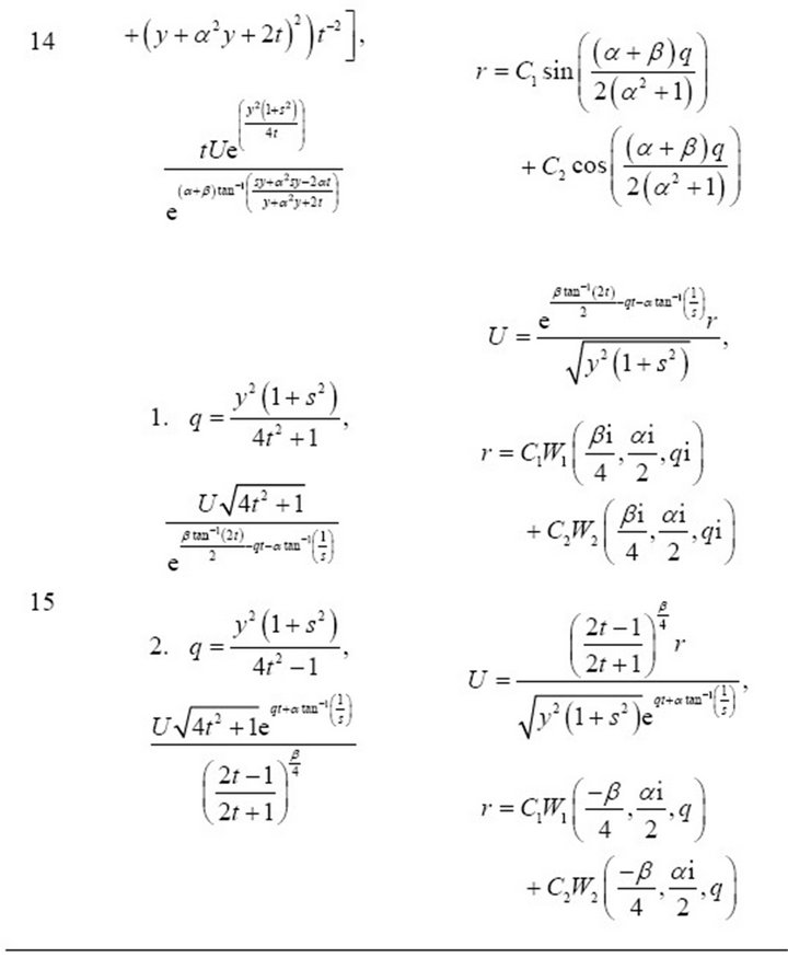
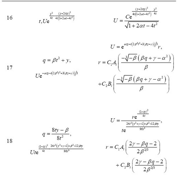
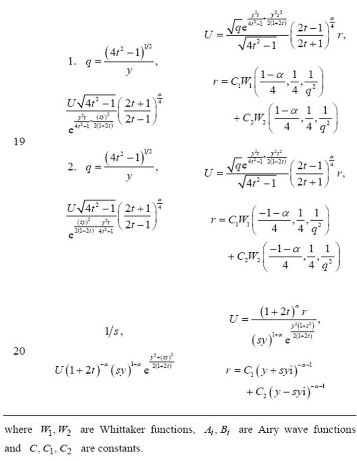
Table 2. Result of invariant solutions of the Equation (1).
8. Acknowledgements
This research is fully supported by the Centre of Excellence in Mathematics, the Commission on Higher Education, Thailand.
REFERENCES
- L. V. Ovsiannikov and A. P. Chupakhin, “Regular Partially Invariant Submodels of the Equations of Gas Dynamics,” Journal of Applied Mechanics and Technics, Vol. 6, No. 60, 1996, pp. 990-999.
- S. Lie, “On General Theory of Partial Differential Equations of an Arbitrary Order,” German, Vol. 4, 1895, pp. 320-384.
- L. V. Ovsiannikov, “Partially Invariant Solutions of the Equations Admitting a Group,” Proceedings of the 11th International Congress of Applied Mechanics, SpringerVerlag, Berlin, 1964, pp. 868-870.
- V. O. Bytev, “Group Properties of Navier-Stokes Equations,” Chislennye Metody Mehaniki Sploshnoi Sredy (Novosibirsk), Vol. 3, No. 3, 1972, pp. 13-17.
- B. J. Cantwell, “Introduction to Symmetry Analysis,” Cambridge University Press, Cambridge, 2002.
- B. J. Cantwell, “Similarity Transformations for the TwoDimensional, Unsteady, Stream-Function Equation,” Journal of Fluid Mechanics, Vol. 85, No. 2, 1978, pp. 257- 271. doi:10.1017/S0022112078000634
- S. P. Lloyd, “The Infinitesimal Group of the NavierStokes Equations,” Acta Mathematica, Vol. 38, No. 1-2, 1981, pp. 85-98.
- R. E. Boisvert, W. F. Ames and U. N. Srivastava, “Group Properties and New Solutions of Navier-Stokes Equations,” Journal of Engineering Mathematics, Vol. 17, No. 3, 1983, pp. 203-221. doi:10.1007/BF00036717
- A. Grauel and W. H. Steeb, “Similarity Solutions of the Euler Equation and the Navier-Stokes Equations in Two space Dimensions,” International Journal of Theoretical Physics, Vol. 24, No. 3, 1985, pp. 255-265. doi:10.1007/BF00669790
- N. H. Ibragimov and G. Unal, “Equivalence Transformations of Navier-Stokes Equation,” Bulletin of the Technical University of Istanbul, Vol. 47, No. 1-2 1994, pp. 203-207.
- R. O. Popovych, “On Lie Reduction of the Navier-Stokes Equations,” Non-Linear Mathematical Physics, Vol. 2, No. 3-4, 1995, pp. 301-311. doi:10.2991/jnmp.1995.2.3-4.10
- A. F. Sidorov, V. P. Shapeev and N. N. Yanenko, “The Method of Differential Constraints and Its Applications in Gas Dynamics,” Nauka, Novosibirsk, 1984.
- S. V. Meleshko, “Classification of the Solutions with Degenerate Hodograph of the Gas Dynamics and Plasticity Equations,” Doctoral Thesis, Ekaterinburg, 1991.
- S. V. Meleshko, “One Class of Partial Invariant Solutions of Plane Gas Flows,” Differential Equations, Vol. 30, No. 10, 1994, pp. 1690-1693.
- L. V. Ovsiannikov, “Isobaric Motions of a Gas,” Differential Equations, Vol. 30, No. 10, 1994, pp. 1792-1799.
- A. P. Chupakhin, “On Barochronic motions of a Gas,” Doklady Rossijskoj Akademii Nauk, Vol. 352, No. 5, 1997, pp. 624-626.
- A. M. Grundland and L. Lalague, “Invariant and Partially Invariant Solutions of the Equations Describing a NonStationary and Isotropic Flow for an Ideal and Compressible fluid in (3+1) Dimensions,” Journal of Physics A: Mathematical and General, Vol. 29, No. 8, 1996, pp. 1723-1739. doi:10.1088/0305-4470/29/8/019
- L. V. Ovsiannikov, “Group Analysis of Differential Equations,” Nauka, Moscow, 1978.
- L. V. Ovsiannikov, “Regular and Irregular Partially Invariant Solutions,” Doklady Academy of Sciences of USSR, Vol. 343, No. 2, 1995, pp. 156-159.
- L. V. Ovsiannikov, “Program SUBMODELS. Gas Dynamics,” Journal of Applied Mathematics and Mechanics, Vol. 58, No. 1, 1994, pp. 30-55.
- S. Khamrod, “Optimal System of Subalgebras for the Reduction of the Navier-Stokes Equations,” Journal of Applied Mathematics, Vol. 1, No. 4, 2013, pp. 124-134. doi:10.4236/am.2013.41022