Applied Mathematics
Vol. 4 No. 4 (2013) , Article ID: 30370 , 20 pages DOI:10.4236/am.2013.44088
3-D Modeling of Axial Fans
1Department of Mathematics and Physics, Lebanese International University, Beirut, Lebanon
2Department of Mathematics and Natural Sciences, American University of Kuwait, Salmiya, Kuwait
3Department of Mathematics and Statistics, University of Windsor, Windsor, Canada
Email: ali.sahili@liu.edu.lb, bzogheib@auk.edu.kw, az3@uwindsor.ca
Copyright © 2013 Ali Sahili et al. This is an open access article distributed under the Creative Commons Attribution License, which permits unrestricted use, distribution, and reproduction in any medium, provided the original work is properly cited.
Received November 12, 2012; revised February 21, 2013; accepted February 28, 2013
Keywords: CFD; Modeling; Mesh Generation; Engine Cooling Fan
ABSTRACT
In this paper we present a full-geometry Computational Fluid Dynamics (CFD) modeling of air flow distribution from an automotive engine cooling fan. To simplify geometric modeling and mesh generation, different solution domains have been considered, the Core model, the Extended-Hub model, and the Multiple Reference Frame (MRF) model. We also consider the effect of blockage on the flow and pressure fields. The Extended-Hub model simplifies meshing without compromising accuracy. Optimal locations of the computational boundary conditions have been determined for the MRF model. The blockage results in significant difference in pressure rise, and the difference increases with increasing flow rates. Results are in good agreement with data obtained from an experimental test facility. Finally, we consider Simplified Fan Models which simplifies geometric modeling and mesh generation and significantly reduce the amount of computer memory used and time needed to carry out the calculations. Different models are compared in regards to efficiency and accuracy. The effect of using data from different planes is considered to optimize performance. The effect of blockage on simplified models is also considered.
1. Introduction
Reference [1] used the commercially available computational fluid dynamics (CFD) code TASCflow3d to integrate the CFD analysis of automotive engine cooling fans in the design methodology and investigated the interaction between aerodynamic and acoustic methodologies. They reported successful application of CFD tools to improve and guide the design of axial flow fans. They also observed good agreement with experiments for the prediction of static pressure gradients at design and high flow rates. They suggested that low flow rate predictions are more sensitive to grid quality. They also found that blade sweeping substantially changes flow patterns and reduces fan efficiency. Further work needs to be done to understand the coupling between blade sweeping and aerodynamic performance.
Using TASCflow, [2] described a CFD based procedure for the design of an automotive engine cooling fan. An investigation of the impact of the numerical schemes available in TASCflow, grid refinement and convergence criterion was accomplished. To validate the procedure, the authors compared computed results to available experimental data and reported good agreement for several test conditions and cascade solidities.
Reference [3] carried out experimental and numerical studies to evaluate CFD models of axial fans. Unlike other investigators, they included the tip clearance in their models. On the experimental side, they collected detailed hotwire measurements in the test facility built at Michigan State University. Two different fans were studied, one was a large truck fan and the other was a mid-sized automotive fan. They reported good results for the larger fan (with higher tip clearance) but not for the other fan (with low tip clearance) where pressure levels were under-predicted, especially at low mass flow rates. Further grid studies and computations with different turbulence models did not bring the performances predicted by the computations closer to the experimental data. The computations without tip clearance and a guided flow inlet lead to smaller losses and consequently to higher pressure rise values.
Reference [4] carried out a numerical analysis using Fluent to compare the MRF and sliding mesh (transient) methods as applied to the analysis of airflow through automotive fans. They showed that there is strong agreement between the results obtained from the two models. From the transient simulation, they obtained the velocity and pressure signals which showed that the peak signal frequencies show strong correlation to the blade passing frequencies and the fan rpm. They suggested that further work needs to be done in order to compare the fan curves with experimental results and to determine the validity of the frequency component due to the fan rpm.
Most simplified fan models are based on one or on a combination of the following theories: the actuator disk theory, the blade element theory and the vortex theory. The actuator disk theory replaces the fan, which has a finite number of blades, with another which has an infinite number of blades. The fan blade loading is distributed over a disk of zero thickness.
In the blade element theory, the blade is divided into a number of blade elements or sections and each section is treated as an isolated two-dimensional aerofoil. It is assumed that the forces on the blade due to its motion through the fluid are dependent only on the aerofoil aerodynamic properties and the relative fluid velocity. These forces are decomposed into normal and tangential forces from which the lift and drag coefficients are determined at the various sections. The influence of the wake and the rest of the fan are contained in the induced angle of attack at the section. Blade element theory provides a lot of details about the flow field, but its treatment of the induced effects is approximate, no account of flow rotation is taken, and the blade loading prediction is not accurate near the blade tip [5].
In the vortex theory, the flow field of the rotor wake is resolved using the fluid dynamic laws that govern the action and influence of vorticity [6]. The fixed wake model uses a vortex sheet that is locally independent of time, and the blade forces are determined using the KuttaJoukowski law. The major shortcoming of this model is that the far wake boundary condition constrains the flow to be parallel to the free stream and does not allow it to diverge. The free vortex model represents the blade by a bound vortex sheet and the wake by force-free shed vortices. The free vortex model captures the fine details of the flow and the transient characteristics of the rotor. However, it is very expensive in terms of computer time.
Reference [7] performed actuator disk experiments and showed that the momentum theory under-predicts the maximum power by up to 10%. This may be largely due to the behavior of the blade tip vortex, which is not accounted for by the theory. This effect is likely even more pronounced when the fan is encompassed by a shroud as in the engine cooling module.
References [8,9] developed a procedure to analyze the flow field and performance of helicopter rotors. The flow was assumed to be steady, laminar, and axisymmetric, and the rotor was represented by point momentum sources distributed along the span of the rotor. Tabulated sectional airfoil data was used to determine the momentum sources which were written as functions of the local flow conditions. The results showed that this model is able to accurately predict the circulation distribution along the span of the rotor blades, the rotor load distribution, the induced velocities in the respective coordinate directions, the integrated performance, and the path of the tip vortex.
Reference [10] developed a three-dimensional numerical method to simulate the asymmetric flow through high-speed low hub-to-ratio blade rows. Compressor blade rows were modeled using actuator disks that provide boundary conditions to the numerical calculation domains. The boundary conditions used are: conservation of mass, conservation of radial momentum, conservation of rothalpy, relative exit flow angle, and entropy rise. A simple choking model was incorporated into the actuator disk boundary conditions based upon two-dimensional flow into a choked section. The author concluded that the method they developed has the capability to faithfully represent the performance of a high-speed rotor for certain flow conditions provided suitable loss and deviation rules and an appropriate choking model are used. In a companion paper [11], the author discussed the application of the above method to the problem of calculating the asymmetric performance of a turbofan operating behind a non-axisymmetric intake and due to the presence of the engine pylon. He reported good agreement with experimental results and with results obtained from three-dimensional simulation of an isolated fan operating with a non-axisymmetric inlet.
The unsteady case was investigated by [12]. These authors used the Gormont model to model the dynamic stall effects on the blade aerodynamic characteristics. This model calculates the dynamic lift and drag coefficients based upon aerofoil characteristics and blade kinematic parameters such as the time derivative of the geometric angle of attack. Comparisons between predicted and measured flapwise bending moments, normal force coefficients and power production were made. They reported that the Gormont dynamic stall model successfully predicts the aerodynamic behavior of the blade tip sections, but fails below 63% span. They suggested that fine-tuning of the empirical constants of the Gormont model should be undertaken in order to improve the accuracy of the predictions. Predicted induced velocity results of the wind turbine operating in yawed flows were in agreement with results based on Glauert’s theoretical analysis. Also, predictions of power production and flapwise bending moments were shown to be close to measurements.
Reference [13] investigated the efficiency of the different pressure interpolation schemes that are available in Fluent for the prediction of HAWTs performances. In the mathematical model that was employed, the flow field around the turbine is described by the incompressible axisymmetric N-S equations. The turbine was idealized as an actuator disk surface on which the blade forces are prescribed according to blade element theory. The authors showed that the pressure interpolation schemes may have significant impact on the computed results. They concluded that the PRESTO scheme is the most promising.
Reference [14] presented an aeroacoustic approach for predicting the noise level generated by an idealized HVAC blower and an axial fan. It is based on a two-step procedure. First, an unsteady flow is computed using AcuSolve to predict aerodynamic sources of noise. Next, an acoustic computation is made using Actran/LA. The variational formulation of Lighthill’s analogy, extended to allow handling control surfaces, is used. They investigated two different approaches for importing aerodynamic sources. An analytic aerodynamic source of compact support was used to study the relative performance of the two approaches. Preliminary acoustic results have been obtained and showed pretty good agreement with experimental results.
Reference [15] studied the performances and flow fields of axial fans with and without a hub leakage between rotor and stator blade rows. Their results indicate that the hub leakage influences the performance of the fan conspicuously and both total pressure and static pressure of the fan are decreased greatly. The hub leakage improves the flow in rotor passages slightly, while significantly deteriorating the flow in the stator passages. Backflow separation and vortices resulting from hub leakage lead to a complex flow structure near the hub in the stator passage.
Reference [16] developed a “downstream flow resistance” (DFR) approach in (STAR-CD) to improve fan performance prediction accuracy with the conventional methods. An experiment-based flow resistance relationship between the flow rate and the pressure drop across the flow resistance creating region of the fan performance test rig is engaged in the downstream area of the computational domain as a region of the distributed resistance. The pressure rise before the flow resistance and the pressure drop across the resistance region are used to iteratively correct and approach the static pressure and flow rate. Using these results, the authors analyzed the inter-blade flow fields. They claimed a great improvement over the conventional method.
The current work is a study of simulation strategies for predicting the aerodynamic performance of two different automotive engine cooling fans. The two fans have the same diameter. Fan1, as shown in Figure 1, has five blades that are forward swept in the direction of rotation. Fan2, as shown in Figure 2, has nine blades with hybrid swept trailing edges and backward swept leading edges. The blades in the fans are radially twisted. The hub radius of Fan2 is larger than that of Fan1, as Fan2 is a high
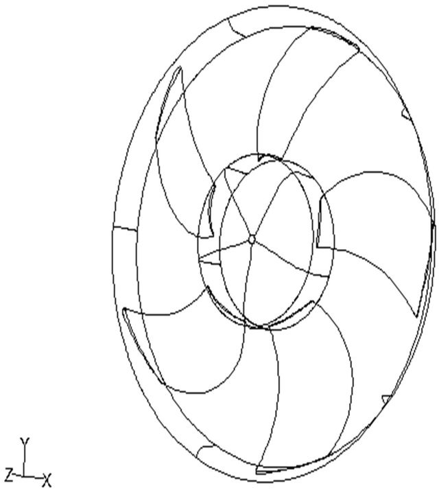
Figure 1. Fan1 geometry.
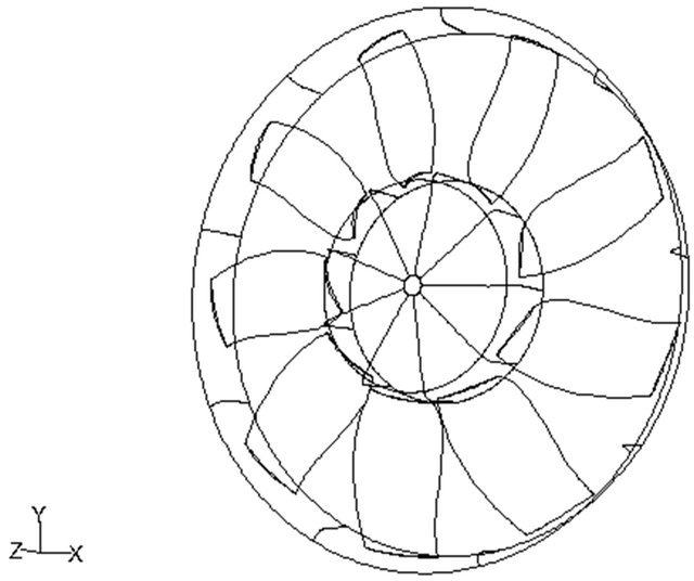
Figure 2. Fan2 geometry.
pressure rise fan and Fan1 is considered to be a low pressure rise fan. Using the CAD module (DDN) of the commercial software ICEM CFD, the geometric models of the fans were built from primitive geometries that consisted of the blades, the hub and ring.
The airflow speed for automobile engine cooling fan applications is low (much lower than the speed of sound). Thus, even though the fluid of interest, air, is a gas, the change in its density through the fan is not significant and we assume that the flow is incompressible. Also, the Reynolds number is not very high; it is in the range of 3 × 10⁴ to 6 × 10⁵.
The experimental data used in this work for the validation of the CFD results were obtained from a test facility established at the University of Windsor. This facility was developed by [17] and used by [18] in his MASc. Thesis. Details about this test facility can be obtained from these works.
2. The Equations of Motion and the Solution Domain
The core computational domain consists of axial extensions upstream and downstream of the fan, extending radially out to the ring as shown in Figure 3. The upstream extension is approximately 1.5 L and the downstream extension is approximately 4.5 L, where L is the
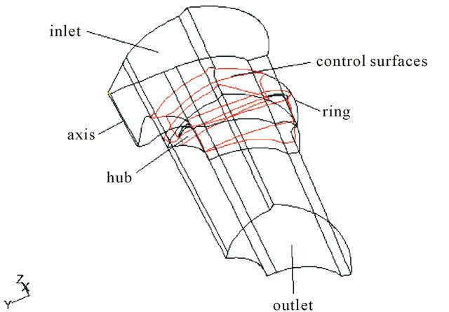
Figure 3. Core computational domain.
height of the hub. Circumferential periodicity is used to reduce the computational domain to one nth (for an nbladed fan) of its full size, greatly reducing the number of cells required for the simulation.
For all the problems considered in this work, we will assume steady, viscous, incompressible, turbulent, and adiabatic flow conditions (heat transfer will not be considered). However, we will deal with three types of problems. The first requires us to solve the equations of motion in a stationary frame of reference, the second requires the employment of a single rotating reference frame (SRF), and the last necessitates the use of a multiple reference frame (MRF), in which part of the domain (referred to as the core part) rotates with the constant angular speed of the fan and the rest of the domain is stationary.
2.1. The Continuity and Momentum Equations
The conservation equations of mass and momentum transfer for fluid flow in an inertial reference frame are presented here.
The equation for the conservation of mass for steady flows, in Cartesian tensor form, can be written as follows:
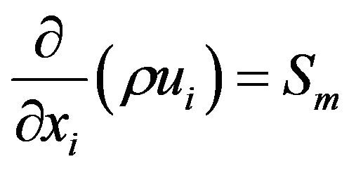 (2.1)
(2.1)
where  is the velocity component in the i direction and
  is the fluid density. The mass source term
  can be used, among other things, to represent any userdefined sources or sinks.
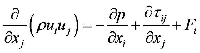 (2.2)
(2.2)
 is the stress tensor and the
  are body forces which may include any modeldependent terms such as user-defined sources.
 The stress tensor  is given by
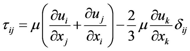 (2.3)
(2.3)
where  is the molecular viscosity, and the second term on the right hand side is the effect of the fluid (volume) dilatation which is proportional to the divergence of the fluid velocity.
2.2. The Rotating Reference Frame
Swirling and rotating flow problems are best solved using rotating reference frames. If the problem at hand is axisymmetric with respect to geometry and flow conditions, the problem may be modeled and solved as a twodimensional problem (which includes the prediction of the circumferential velocity). However, if there are geometric changes and/or flow gradients in the circumferential direction, a three-dimensional rotating model is needed. In such flows the coordinate system is moving with the rotating equipment and thus experiences a constant acceleration in the radial direction. Therefore, the rotating reference frame is a non-inertial coordinate system.
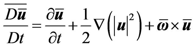
The continuity equation is invariant under the transformation that takes us from the inertial system to the non-inertial system and vice versa. The momentum equations, on the other hand, are not invariant because of the acceleration terms. The momentum equation can be written as
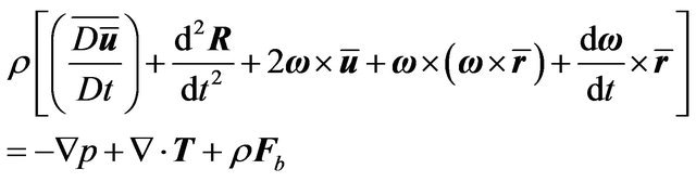
where T is the viscous stress tensor. The acceleration term can be written as
Since only spatial derivatives are involved in the del operator, the gradient of a scalar and the divergence and curl of a vector are invariant. Hence the right hand side of the momentum equation is the same in both systems.
2.3. Boundary Conditions
The solution of the equations of motion for any specific flow problem cannot be obtained without the prescription of appropriate auxiliary conditions, a set of initial and boundary conditions. Since the problem we are concerned with is a steady-state problem, initial conditions are not relevant. Boundary conditions are values of the dependent variables that are specified at the boundaries of the fluid domain. Because of viscosity, the relative velocity between the fluid and a solid wall is zero. This is the no-slip condition for viscous fluids. Since  is the absolute velocity of the fluid, this condition means that
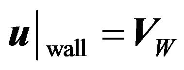
where  is the absolute velocity of the wall. If the wall is at rest, then
 , and the wall boundary condition becomes
where  is the local unit tangent vector in any direction on the surface of the wall and
  is the unit normal on the wall surface. Here,
  and
and  are the tangential and normal components, respectively, of the fluid velocity
  on the wall.
Sometimes it may be appropriate to impose the slip boundary condition at a solid wall even though the flow in general is viscous. In this case the fluid is treated as inviscid, and boundary condition on this wall becomes
 , and
, and 
This condition is also referred to as the zero shear stress wall boundary condition. If two walls form a periodic pair then, for any flow variable , the condition that must be imposed is

The axis boundary type must be used as the centerline of an axisymmetric geometry. It can also be used for the centerline of a cylindrical-polar quadrilateral or hexahedral grid. To determine the appropriate physical value for a particular variable at a point on the axis, the cell value in the adjacent cell is used. A" velocity distribution is specified at the inlet, and at the outlet the condition of radial pressure distribution is specified. At the inlet,  is always negative indicating that the flow is into the flow domain.
2.4. Turbulence Modeling
Most fluid flows encountered in engineering practice are turbulent, and certainly this is the case in turbomachinery flows. To this date, there is no single turbulence model that is best for all classes of problems. The choice of a model for a specific problem depends on many factors such as the physics of the flow under consideration, the level of accuracy required, the available computational resources, and the amount of time available for the simulation. In this work we use the standard  model which is the most widely used and validated turbulence model. The standard
  model is a semi-empirical model and focuses on the mechanisms that affect the turbulent kinetic energy and its dissipation rate
  [19].
[19].
The transport equations for k and  are
are
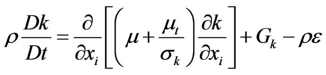
and
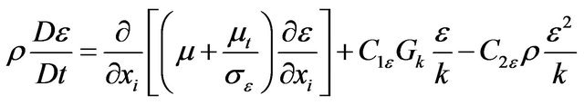
where  represents the generation of turbulent kinetic energy due to the mean velocity gradients and is given by
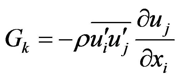 .
.
where  represents the velocity fluctuations from the mean, and overbar indicated Reynolds averaged quantities.
The “eddy” or turbulent viscosity is computed from
 .
.
In these equations,  ,
,  and
and  are constants determined from experiments.
  and
and  are the turbulent Prandtl numbers for k and
 , respectively.
3. Mesh Generation
All meshing related to this work is accomplished using the ICEM/Hexa grid module from ICEM CFD Engineering [20]. One of the most important capabilities of Hexa is elliptic smoothing. Mesh generation is an integral part of any numerical scheme, and the quality of the mesh affects both the accuracy and stability of the numerical computation. The properties associated with mesh quality include smoothness, grid point clustering, cell shape, and orthogonality.
Since the continuous physical domain is represented by a discrete mesh, the degree to which the salient features of the flow (such as shear layers, separated regions, and boundary layers) are resolved depends on the density and distribution of nodes in the mesh. Poor resolution in regions with strong flow gradients can dramatically alter the flow characteristics. For example, the prediction of separation due to an adverse pressure gradient depends heavily on the resolution of the boundary layer upstream of the point of separation. The proper resolution of the boundary layer (i.e., mesh spacing near walls) also plays a significant role in the accuracy of the computed wall shear stresses. Numerical results for turbulent flows tend to be more susceptible to grid dependency than those for laminar flows because of the strong interaction of the mean flow and turbulence. For the standard  turbulence model with wall functions, the distance from the wall to the adjacent cells is determined by [21]
where  and
and  are the density and kinematic viscosity of the fluid, respectively, y is the distance from the wall,
  is the friction velocity, defined as
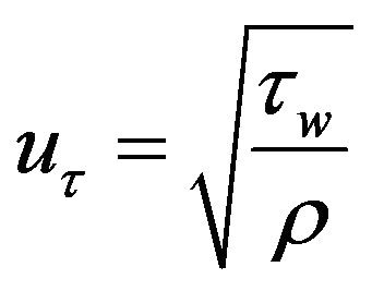
and  is the wall shear stress. It is known that the loglaw is valid for
 . Using of excessively fine mesh near the walls should be avoided, because the wall functions cease to be valid in the viscous sublayer [21]. However, every flow passage should be represented by enough cells to adequately resolve the flow field in that passage. In regions of large gradients, as in shear layers or mixing zones, the grid should be fine enough to minimize the change in the flow variables from cell to cell.
The skewness and aspect ratio of a grid cell also have a significant impact on the accuracy of the numerical solution. Skewness can be defined as the difference between the cell’s shape and the shape of an equilateral cell of equivalent volume. Highly skewed cells can be tolerated in benign flow regions, but can be very damaging in regions with strong flow gradients, as they can decrease accuracy and destabilize the solution. Aspect ratio is a measure of the stretching of the cell. Quadrilateral/ hexahedral elements obtained by structured meshers permit a much larger aspect ratio than triangular or tetrahedral cells obtained by unstructured meshers. A large aspect ratio in a triangular/tetrahedral cell will invariably affect the skewness of the cell, and that may impede accuracy and convergence as mentioned above.
Orthogonality in the interior domain is related to skewness. The less skewed the cells are, the more orthogonal the mesh is said to be. Orthogonality is particularly important at surfaces, because it simplifies and makes more accurate the computation of normal gradients.
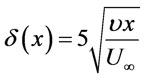
To ensure a high quality mesh that possess all of the above features, we create control surfaces around the blade profile, and divide the solution domain into many blocks in order to generate a multi-block structured mesh. To make sure that we have enough cells within the boundary layer, an estimate of the boundary layer thickness is needed. Based upon the Blasius solution for laminar flow over a flat plate at zero incidence [22]
Taking , the average radius,
  where
where  is the rotational speed (=2300 rpm), and
 ![]() = 0.000017894, we get
= 0.000017894, we get
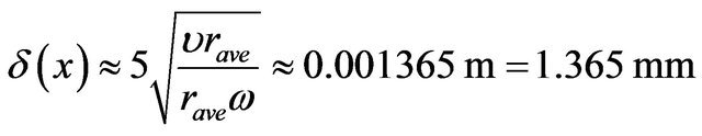 .
.
Considering this estimate of the boundary layer thickness, the first grid point off a wall is placed at less than 0.3 mm from the wall in the core meshes for all fans. Owing to greater energy losses, turbulent boundary layers grow faster than laminar ones and are generally thicker [23], thus sufficient grid clustering near a wall is guaranteed once it is guaranteed for laminar boundary layers. However, rotating boundary layers may be very thin, and a very fine grid is needed near rotating walls. In addition, swirling flows will often involve steep gradients in the circumferential velocity, for example near the centerline of a free vortex type flow, and thus require a fine grid for accurate resolution. Another way of stating the problem is to say that, for laminar flows, the distance from the wall of the first grid point,  , must obey the formula [21]:
Because of the large changes in flow direction which occur, coupled with the need to satisfy periodic boundary conditions, fan flow calculations are extremely demanding in terms of grid definition. The periodicity condition demands that all flow properties at corresponding points one blade pitch apart must be identical, and to achieve this, the grid points on each periodic pair of surfaces must be rotational copies of each other. Thus maintaining orthogonality becomes a challenging task. To improve mesh orthogonality and reduce skewness, control surfaces have been introduced around the blade, and the flow passage is divided into many blocks which resulted in high quality meshes. Figures 4 and 5 show the grid distribution on the hubs of Fan1 and Fan2, respectively. Hexa provides quantitative methods for checking the quality of the mesh. The determinant checks the deformation of the cells in the mesh using a test that computes the Jacobian of each hexahedron and scales the determinant of the matrix in such a way that 100 is a perfectly regular cell, zero is degenerate in one or more edges, and negative values indicate inverted cells. In general, values above 0.25 are acceptable for most solvers. For our calculations, the minimum determinants for the meshes of Fan1 and Fan2 are 0.25 and 0.45, respectively. The low value of the determinant mainly exists in the region near the axis boundary, a very small cylinder surface connecting the inlet and the hub, where the mesh cells are numerous and have very small circumferential edges. However, since these cells are located in a stagnant, or almost stagnant region, the shape of these cells does not have a significant impact on the converged solution. The angle check computes the maximum internal angle deviation from  for each cell. Minimum angles of 9 and 4.5 degrees
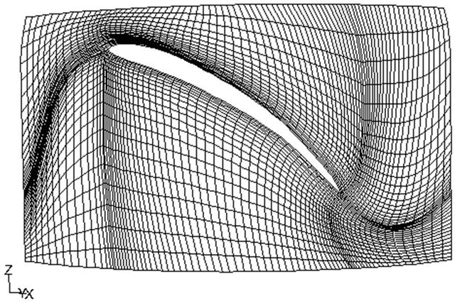
Figure 4. Grid on hub of Fan1.
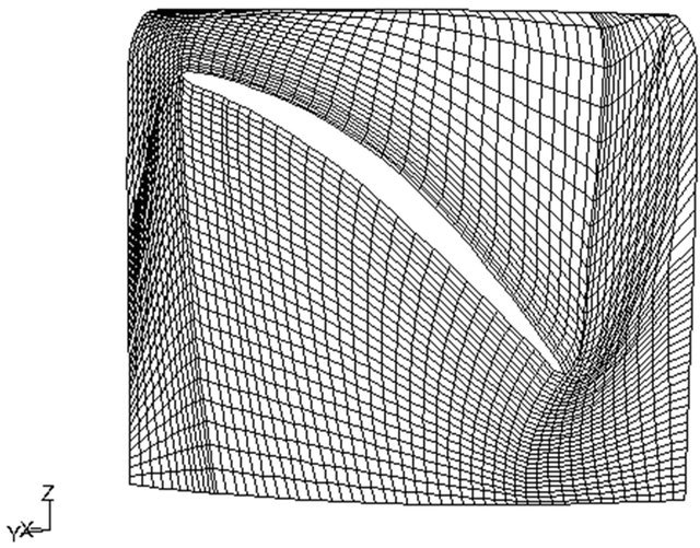
Figure 5. Grid on hub of Fan2.
correspond to Fan1 and Fan2, respectively. The extension to the core mesh does not pose any difficulties for meshing because of the simple geometry of the extensions. After merging the core mesh with the extensions, it is recommended that contiguous surfaces be fused for MRF calculations so that contiguous nodes become identical.
Grid Dependency Analysis
To check the solution for sensitivity to the mesh used, the grid was refined according to both pressure and velocity magnitude gradients. Solution adaptive refinement of the mesh adds cells where needed, which allows for the features of the flow field to be better resolved. If the original mesh is not the best possible, the refined mesh is optimal for the flow solution because the solution is used to determine where more cells are to be added.
For velocity gradient adaption, most of the cells that were refined were on solid walls such as the blade, hub and the ring, and the number of nodes increased by about 11%. When adaption was carried out based on pressure gradient, more cells in the interior of the domain were refined, and it was performed such that the resulting refined mesh is of the same size as the velocity-gradient based refined mesh.
It was found that no significant changes due to the refinement of the mesh occur in the flow field. Also, contours of pressure, velocity magnitude and all the velocity components were checked on the plane 25 mm downstream of the fan, and all plots were virtually identical for both the original and refined meshes. Pressure seems to be more sensitive to grid adaption, but the maximum difference is about 8%. The number of iterations increased significantly for the refined grid with pressure gradient based adaption but decreased slightly with velocity gradient based grid adaption.
4. CFD Formulation and N-S Solver
The CFD software Fluent was used to numerically solve the equations of motion. Fluent’s solver employs a Cartesian coordinate system . For our purposes, and for turbomachine calculations in general, the natural choice of coordinate system would seem to be the cylindrical system
  centered on the axis of rotation. However, a Cartesian system is still preferable because it simplifies the calculations at the interior mesh points, although it complicates the application of boundary conditions. The major problem with using cylindrical coordinates is that the direction of the radial vector changes around the surfaces of the cells which affects the evaluation of radial components of the flow variables [23].
Two numerical methods are available in Fluent, the coupled solver and the segregated solver. Both use a control-volume-based technique to convert the governing equations to algebraic equations that can be solved numerically. In the segregated solver approach, the governing equations are solved sequentially. Because the governing equations are nonlinear, an iterative procedure is used to solve them. Each iteration consists of the following steps:
1) Fluid properties are updated based on the current iteration step. For the first step, the fluid properties are updated based on the initialized solution;
2) The momentum equations are solved using current values for pressure and face mass fluxes, in order to update the velocity field;
3) The velocities obtained in step 2 may not satisfy the continuity equation locally. A Poisson-type equation for the pressure correction is used to obtain the necessary corrections to the pressure and velocity fields and the face mass fluxes;
4) Equations for turbulence scalars are solved using the updated values of the other variables;
5) Convergence is checked.
These steps are repeated until the convergence criteria are met.
4.1. Discretization of the Governing Equations
First order discretization may be acceptable when the flow is aligned with the grid because it generally yields better convergence than second order. However, when the flow is not aligned with the grid, first order convective discretization increases the numerical diffusion and, in this case, second order is recommended. For most of our calculations, we choose the second order scheme for the momentum equations and the first order scheme for the rest of the governing equations. Upwind differencing eliminates the need for knowing velocities downstream, and hence the exit boundary conditions are not needed to solve the problem, that is, the velocity at the outlet is not specified as a boundary condition, and this allows the flow through the fan to diverge naturally. The adequacy of the central differencing scheme is governed by the nondimensional cell Peclet number  which is defined by
where  is the cell width. When
  physical diffusion will be sufficient to counteract local convective instabilities in regions with large velocity gradients. For
  the convective insensitivity of central differencing leads to the appearance of oscillations in the solution. To calculate the convective and diffusive fluxes, this scheme introduces influencing at the cell center from the directions of all its neighbours. Thus for high
 , the flow direction is not identified and the strength of convection relative to diffusion is not recognized [19]. Because of the restriction on the Peclet number, central differencing discretization is not suitable for high Reynolds number flows, or if the grid is coarse. For general purpose flow calculations other discretization schemes are preferred, such as second order upwind or the QUICK schemes.
The quadratic upwind interpolation for convective kinetics (QUICK) scheme uses a three-point upstreamweighted quadratic interpolation for cell face values [24]. It has been found that the QUICK scheme generally yields much better convergence and predicts a lower pressure than the second order scheme.
The discretized form of the x-momentum equation, for instance, can be written as
Since pressure and velocity are both stored at cell nodes, an interpolation scheme is needed to compute the face values of pressure,  , appearing in equation the above.
Two of the several pressure interpolation schemes that are available in FLUENT were implemented in our calculations. The STANDARD scheme interpolates the pressure values at the faces using momentum equation coefficients [24]. This works well when the pressure variation between cell nodes is smooth. If, as is the case with strongly swirling flows, there are jumps or large gradients in the momentum source terms between control volumes, the pressure profile will have high gradients at the cell face. The above scheme cannot be used to interpolate pressure, else a discrepancy will show up as overshoots or undershoots in the cell velocity. The PRESSURE Staggering Option (PRESTO) uses the discrete continuity balance for a staggered control volume about the face to compute the face pressure [25]. This procedure is similar in spirit to the staggered grid schemes used with structured meshes, and it may only be used with quadrilateral and hexahedral meshes.
For incompressible flows the density is constant and hence not linked to the pressure. There are several algorithms that establish such a link. In this work the required link is accomplished using the SIMPLE (Semi-Implicit Method for Pressure Linked Equations) algorithm [25], which uses a relationship between velocity and pressure corrections to the effect that if the correct pressure field is applied in the momentum equations, the resulting velocity field should satisfy the continuity equation.
4.2. Numerical Boundary Conditions
The importance of imposing physically realistic, wellposed boundary conditions cannot be overemphasized. The fluid flow inside a CFD solution domain is driven by boundary conditions and, in a sense, the solution process is nothing but the extrapolation (based on the flow equations) of the boundary data into the domain interior. The imposition of improper or unrealistic boundary conditions is the most common cause of divergence of CFD simulations [3,4]. Even if the solution converges, incorrect boundary conditions will certainly result in an incorrect solution. Various kinds of boundary conditions are used for CFD computations. The following are most common and are relevant to the calculations performed in this study.
4.2.1. Flow Inlet
At an inlet boundary, all quantities must be prescribed. In our calculations we used the velocity-inlet boundary condition to define the velocity and scalar properties of the flow at the inlet of the domain. This achieves two goals. First, it simulates the ram effect of the air that would be caused by the automotive vehicle motion. For every value of inlet velocity there is a corresponding volume flow rate (Q) where
Also, the inlet velocity is used to initialize the velocity field in the whole solution domain.
4.2.2. Flow Outlet
At the domain outlet we usually do not know much about the flow. Therefore, in order to prevent errors from propagating upstream, outlet boundary conditions should be placed as far downstream of the region of interest (the fan, for example) as possible. In our calculations pressure outlet boundary condition was used to define the static pressure distribution (and other scalar variables) at flow outlets. The pressure outlet boundary condition often results in a better rate of convergence than other outflow boundary conditions.
4.2.3. Solid Wall
Two kinds of wall boundary conditions are used. The no-slip boundary condition is used on the blades, the downstream hub extension (the shaft), and the outer cylinder of the downstream extension. This is obviously the natural condition in viscous flows. However, if the wall is a numerical boundary that does not exist in the physical domain, it may be more appropriate to apply a different wall boundary condition. In our calculations we apply a slip wall condition to the upstream outer cylinder by specifying zero shear stress at this wall.
4.2.4. Periodic Planes
Periodic boundary conditions can be used to take advantage of special geometrical features of the solution domain. If it is expected that the flows across two (periodic) planes are identical, then the flow conditions at one plane are used to calculate the flow through the other. In the CFD modeling of fans there is, in general, no need to model the whole solution domain since it is expected that the flow will be periodic with periodic boundaries cutting through flow passages. Hence, only one nth of the domain of an n-bladed fan needs to be modeled.
4.2.5. Far-Field Surface
If the far-field boundary is located far enough away that it does not influence the flow properties in the interior domain, then free-stream conditions are imposed. Otherwise, appropriate boundary conditions need to be applied. In our simulations, the inlet, outlet and the outer radial extensions are far-field type boundary conditions, and their locations are shown to have a significant influence on the flow field, as will be seen later.
4.2.6 Axis Boundary
At the axis boundary condition the physical value for a particular flow variable is determined using the cell value in the adjacent cell. The fan axis in our calculations is taken as a long cylindrical tube with a very small diameter and extending from the center of the fan hub to the inlet.
4.3. Turbulence Parameters
Boundary conditions for the turbulence equations are also needed at the inlet and outlet. This could be done by specifying k and  distributions at the inlet/outlet, or, in problems where inflow occurs, such as the one we are concerned with, it may be appropriate to specify uniform values. However, it is also possible to specify more convenient turbulence quantities such as intensity and length scale. Experimental data is the best source for obtaining estimates of turbulence parameters, but such data is rarely available for CFD users. Another source could be the relevant literature, else crude approximations can be obtained by means of simple assumed forms. More details can be found in [19,21].
5. Results and Discussion
5.1. The Core Domain
In Figure 6, which presents velocity magnitude contours on a meridian plane that cuts through the blade of Fan1, a stagnant flow region appears near the axis of the fan. The whole region that extends radially outward from the axis to the hub radius and axially from the hub to the inlet is a very low velocity region, which suggests that it may be possible to completely ignore this region in the simulation of the fan. A detailed analysis of this model is presented in this section.
The top of the hub is removed and the hub is replaced by a long cylinder extending upstream to the inlet boundary. As a result it is much easier to build the mesh since the domain is much simpler. This model is referred to as the “hubless” fan. Previous fan simulations have incorporated this assumption (eg. [1]) but its validity and advantages have not been discussed.
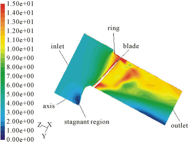
Figure 6. Contours of velocity (Fan1, Qd, 2300 rpm).
To study this simplified configuration more closely we compare simulation results to those of the original core domain. Figures 7 and 8 show that it yields a very reasonable fan pressure rise for both fans and all working conditions.
For Fan1, design condition, the pressure distribution on the pressure surface and the relative velocity angle on the suction surface are unaltered in the new configuration (Figures 9 and 10).
Also, pressure and velocity contours on the blades and on horizontal planes 20 mm downstream of the fan are very similar. For the high flow rate, the relative velocity angle is in good agreement (Figure 11), but some discrepancy in the radial distribution of circumferentially averaged pressure is evident (Figure 12). The same observation can be drawn from pressure contours. The
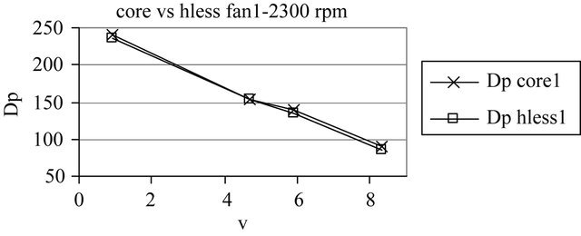
Figure 7. Pressure rise curves for Fan1, 2300 rpm.
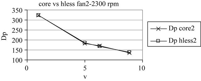
Figure 8. Pressure rise curves for Fan2, 2300 rpm.
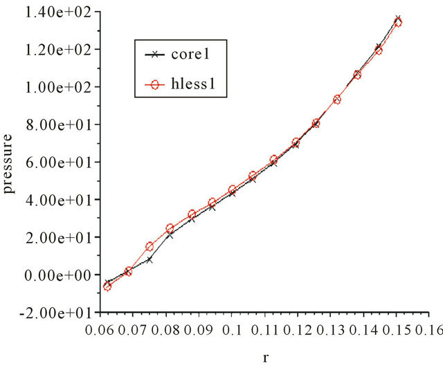
Figure 9. Static pressure vs radius on the pressure surface (Fan1, Qd, 2300 rpm).
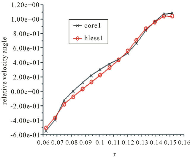
Figure 10. Relative velocity angle vs radius on the suction surface (Fan1, Qd, 2300 rpm).
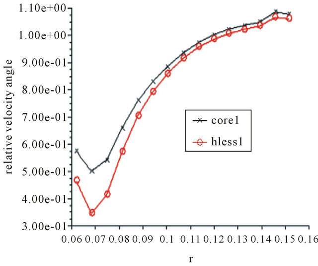
Figure 11. Relative velocity angle vs radius on the suction surface (Fan1, 1.8Qd, 2300 rpm).
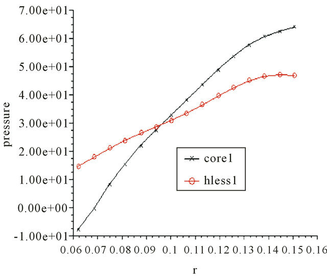
Figure 12. Static pressure vs radius on the pressure surface (Fan1, 1.8Qd, 2300 rpm).
boundary layer doesn’t change significantly but the wake behind the blades widens. At the low flow rate, the radial distribution of the relative velocity angle changes significantly, and pressure contours on the blade are quite different.
For Fan2, 0.299 m3/s case, the relative velocity angle agreement is good as can be seen from Figure 13. The circumferentially averaged radial pressure distributions on the blade surface compare well (Figures 14 and 15), and no changes to boundary layer structure are evident.
Velocity magnitude contours compare reasonably well on the plane z = −20 mm, although the hubless model exhibits stronger circumferential uniformity than the model with the hub. For the high flow rate, the relative velocity angle is in good agreement, and the circumferentially averaged radial pressure distributions on the blade are almost identical. For the low flow rate the pressure contours on the lower blades are identical. The contours of relative velocity magnitude on a radial plane at midspan are very similar, and the oil flow patterns on the suction surfaces are almost identical.
5.2. The Multiple Reference Frame Model
The core domain model tends to over-predict the fan pressure rise and, of course, confines the flow downstream of the fan, not allowing it to expand beyond the outer ring radius. Hence, it does not provide a very realistic model of the fan test facility. In order to accurately simulate the experimental facility, the core domain is extended in both the radial and axial directions. Since the box is very large compared to the fan, the interior of the box far away from the fan has virtually no flow. So, in our numerical model, the solution domain has been made smaller than the real physical domain, and instead of rectangular outer walls, a cylindrical surface has been
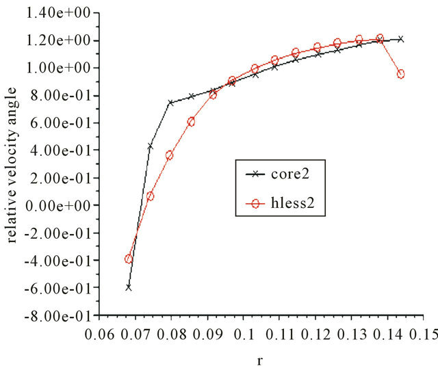
Figure 13. Relative velocity angle vs radius on the suction surface (Fan2, Qd, 2300 rpm).
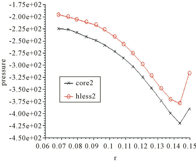
Figure 14. Static pressure vs radius on the suction surface (Fan2, Qd, 2300 rpm).
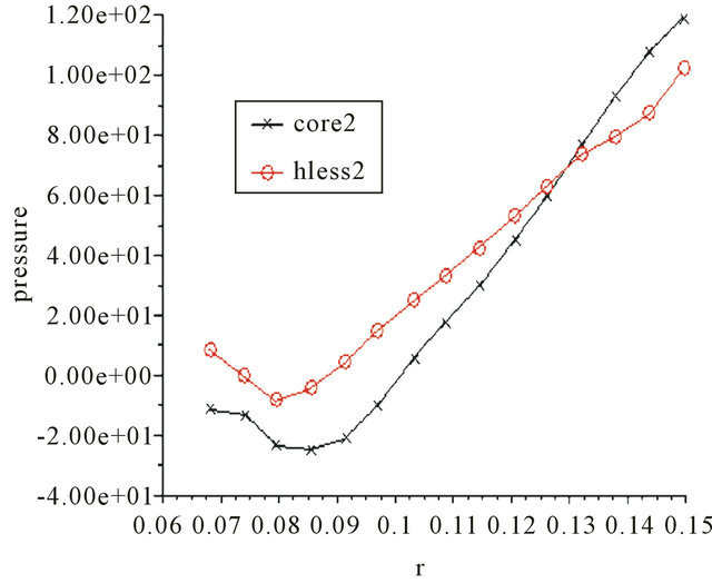
Figure 15. Static pressure vs radius on the pressure surface (Fan2, Qd, 2300 rpm).
created as an outer boundary for the numerical model. The location of the upstream and downstream outer boundaries cannot, however, be completely arbitrary. To study the effect of the location of these computational boundaries on the pressure rise through the fan and on the flow behind it, three different configurations have been tested. Configuration A has larger upstream (approximately five fan diameters) than downstream (approximately three fan diameters) radial extensions (Figure 16). The radial extensions for Configuration B are opposite to A, i.e. the upstream is smaller than the downstream. Configuration C has upstream and downstream of equal size, approximately three fan diameters. For each fan, all configurations have the same mesh as in the core domain model and the same axial lengths, about 55 blade axial lengths upstream and 80 downstream of the fan. Also, since the flow behind these fans is usually obstructed by a large object, such as the engine block, it is important to study the effects of such a blockage on the fan performance. The results presented in this part of the investigation pertain to Fan1.
In the numerical test facility, the fan covers only a very small portion of the overall solution domain, and if the rotating reference frame is applied in the outer region, a large Coriolis force will dominate the solution, masking out important physical forces such as the viscous force in the region near the fan. Other problems may arise if the whole solution domain is considered in a rotating reference frame. For instance, the flow is known to be highly three-dimensional, but, in general, rotation imparts some kind of rigidity to the flow which results in a strong tendency of the flow towards two-dimensionality. Also, rotation confers some elasticity on the fluid that makes possible the propagation of waves in a rotating fluid [26]. Thus, in the present simulations, the outer region of the computational domain is kept stationary and only the core region is allowed to rotate.
The results of the numerical simulations of the fan at 2300 rpm are compared with data from the test facility [17]. Figure 17 shows that the predicted pressure rise varies significantly depending upon the location of the outer boundary condition. Configurations A and C both have good agreement with experimental data. The core mesh simulation discussed in Section 5.1 (referred to here as Configuration D) significantly over-predicts the pres-
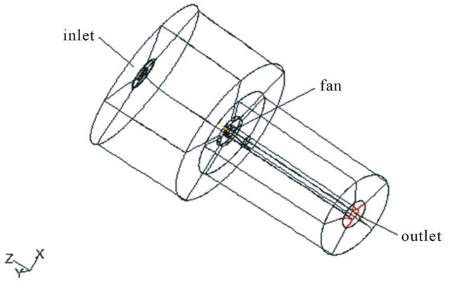
Figure 16. Computational domain: Configuration A.
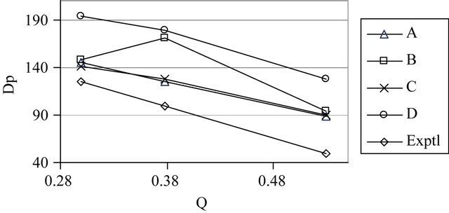
Figure 17. Pressure rise (Pa) vs flow rate (m3/s) A: larger upstream plenum; B: smaller upstream plenum; C: same size large plenums; D: core mesh.
sure rise. Configuration B does not correctly predict the pressure rise vs flow rate trend. The same trend is observed for the 2700 rpm case.
For Configuration B, the predicted velocity field is also incorrect.
Plots of typical velocity magnitude contours are shown in Figures 18-28, on planes 30 mm upstream, 25 mm and 100 mm downstream of the fan, respectively. As can be observed from the upstream velocity magnitude contours in Figures 18-20, Configuration B appears to model the upstream region as accurately as the other configurations. The contours for Configuration C are essentially the same as those for A.
Even though the pressure is poorly simulated in B, the experimental and numerical contours are in good agreement on a plane immediately behind the fan, as illustrated in Figures 21-24 by comparing Configurations A and B with the experimental results. All configurations, except the core domain, have similar contour plots, although the spread between minimum and maximum speed is slightly greater for Configuration B. The simulations for A and B tend to smear out the high velocity regions and move them closer to the hub but, in general, these contours are in good agreement with the experimental contours on planes close to the fan. Configuration D, which confines the flow so that it cannot expand beyond the outer ring, does not accurately simulate the flow downstream of the fan. (The contours for Configuration C are the same as those for A).
Figures 25-28 show the velocity magnitude contours at 100 mm downstream of the fan, on an annulus with outer radius slightly beyond the ring radius. These illustrate that the numerical predictions from Configurations B and D are completely inaccurate. The predicted velocity magnitude is too low, falling completely out of the experimental range in both cases. Configuration C gives slightly more accurate results than A on this annulus, although the high velocity region is located further from the shaft than is observed in the experiments.
Figures 29 and 30 show the contours on an expanded annulus at 100 mm downstream. For Configuration A (C is similar), there is very good agreement between the experimental and numerical contours, but the predicted flow has expanded about 25 mm (16%) beyond the outer ring. The simulation for Configuration B suggests that the downstream flow expands widely, about 72% more than in the test facility. Furthermore, the speed is entirely out of the experimental range. The importance of the location of the numerical boundary conditions is also seen to have a drastic influence on the predicted downstream static pressure.
5.3. Effects of Blockage
The blockage imposed by the engine is modeled as a solid cylinder with radius equal to the radius of the fan ring,
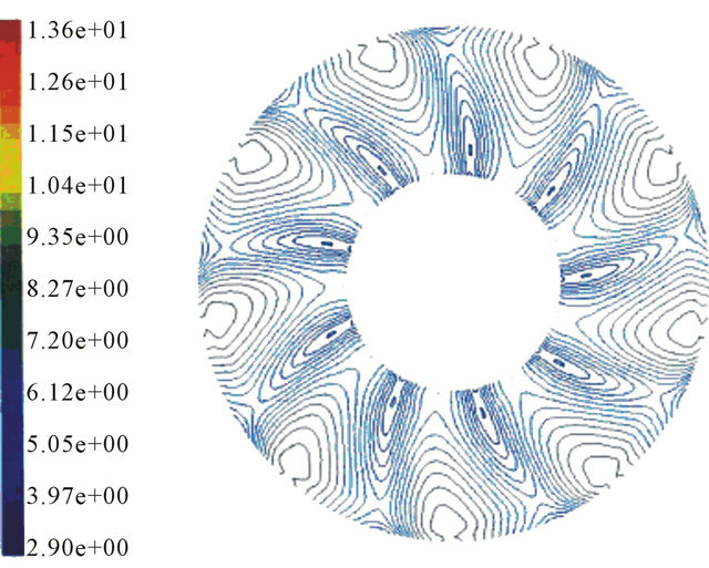
Figure 18. Velocity magnitude on a plane 30 mm upstream of Fan2 (Configuration A).
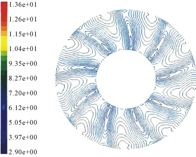
Figure 19. Velocity magnitude on a plane 30 mm upstream of Fan2 (Configuration B).
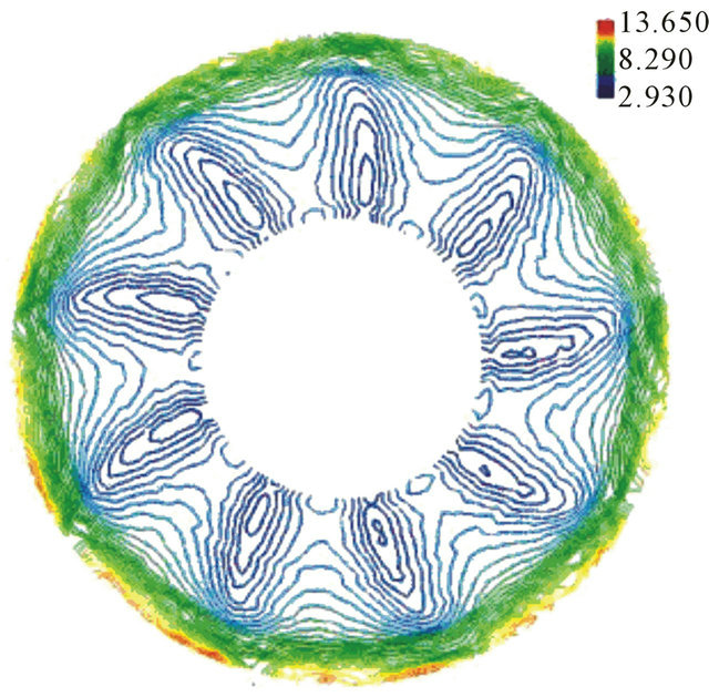
Figure 20. Velocity magnitude on a plane 30 mm upstream of Fan2 (Experimental).
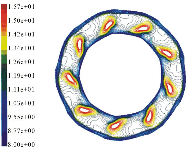
Figure 21. Velocity magnitude on a plane 25 mm downstream of Fan2 (Configuration A).
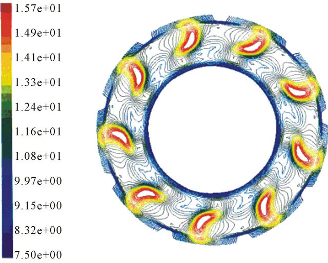
Figure 22. Velocity magnitude on a plane 25 mm downstream of Fan2 (Configuration B).
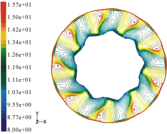
Figure 23. Velocity magnitude on a plane 25 mm downstream of Fan2 (Configuration D).
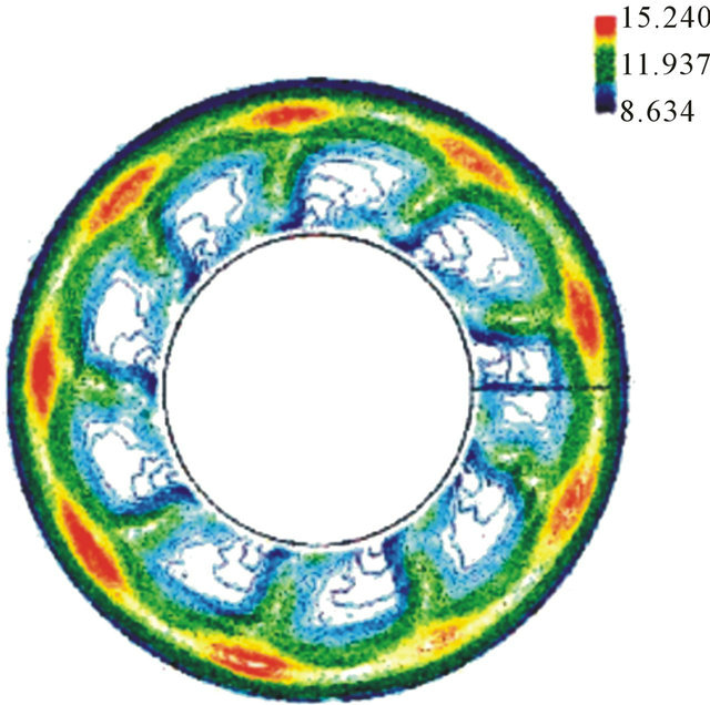
Figure 24. Velocity magnitude on a plane 25 mm downstream of Fan2 (Experimental).
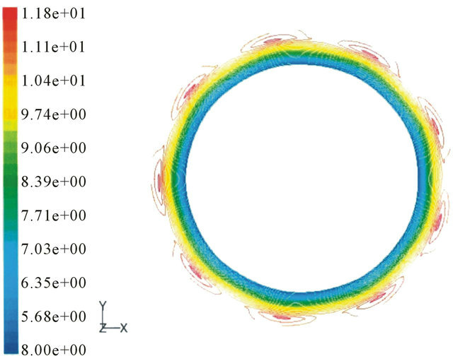
Figure 25. Velocity magnitude on a plane 100 mm downstream of Fan2 (Configuration A).
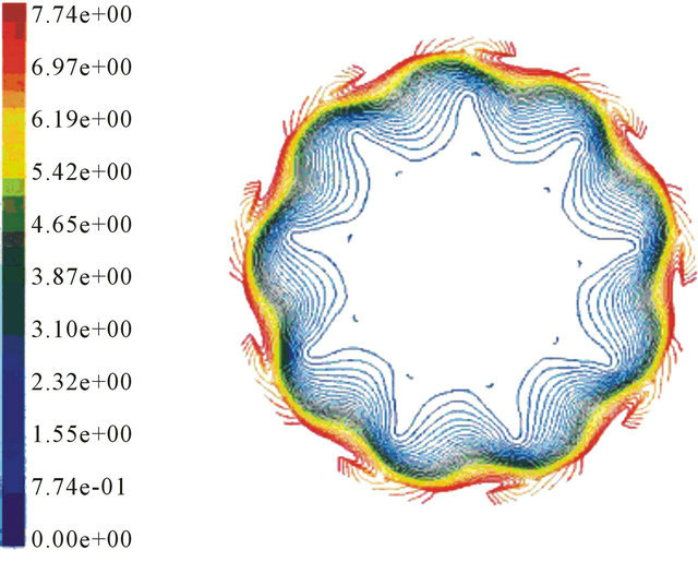
Figure 26. Velocity magnitude on a plane 100 mm downstream of Fan2 (Configuration B).
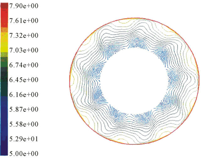
Figure 27. Velocity magnitude on a plane 100 mm downstream of Fan2 (Configuration D).
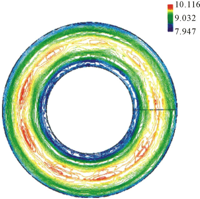
Figure 28. Velocity magnitude on a plane 100 mm downstream of Fan2 (Experimental).
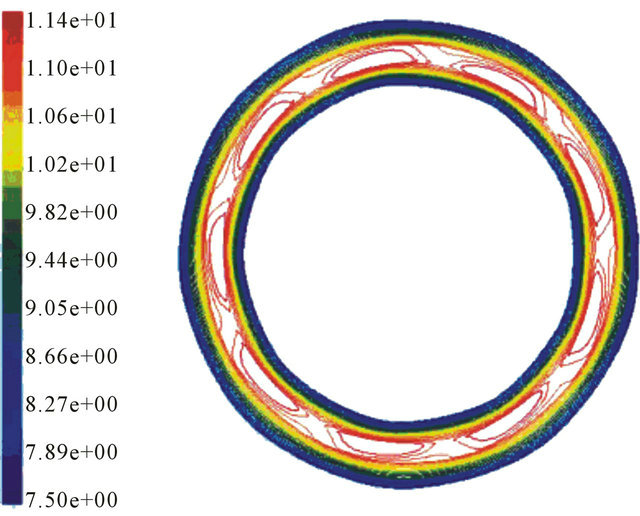
Figure 29. Velocity magnitude on an annulus 100 mm downstream of Fan2 (Configuration A, 25 mm expansion).
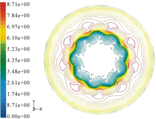
Figure 30. Velocity magnitude on an annulus 100 mm downstream of Fan2 (Configuration B, 115 mm expansion).
placed 50 mm downstream of the fan and extending to half the downstream length of the computational domain (Figure 31). The inclusion of such a blockage is important since it simulates the engine that blocks the flow of air behind the fan in any underhood configuration.
Figure 32 shows pressure rise vs velocity for the 2300 rpm rotational speed. As expected, there is a significant difference in pressure rise in the presence of the blockage, and the difference increases with increasing flow rates. This is useful information since some simplified fan models require a priori knowledge of pressure rise as a function of flow rate or velocity. Some simplified fan models replace the fan with a source zone inside which the forces exerted by the fan blades on the fluid are applied. Therefore, it is important to know how these forces are affected by the presence of the blockage. It has been shown that the blade forces show an increase of 8%, 15% and 4%, in the x, y, and z directions, respectively.
Since the data needed for the development of the various boundary condition models that are discussed in the next section is taken from the plane at 5 mm downstream of the fan, we look at typical velocity magnitude contours on this plane for the unblocked and blocked full CFD simulations in Figures 33 and 34. The flow is seen to expand due to the blockage and the higher values of the velocity magnitude shift to the outer ring and coincide with the blade tips. Results also show that the blockage causes the flow near the hub to expand, and higher axial velocities appear beyond the ring. The blockage pushes the flow outward, significantly increasing the radial component of the velocity field (Figure 35). The tangential velocity profile also changes significantly with an increase in the last 2/3 of the fan region.
6. Simplified Fan Models
One of the most widely used simplified fan models in industry is a variant of the actuator disk model which is also available in most commercial CFD software, such as Fluent. In this model, the fan is replaced by an infinitely thin surface on which pressure rise across the fan is specified as a polynomial function of normal velocity or flow rate. The advantages of this model are that it is simple, it accurately predicts the pressure rise through the fan and the axial velocity, and it is robust. However, this
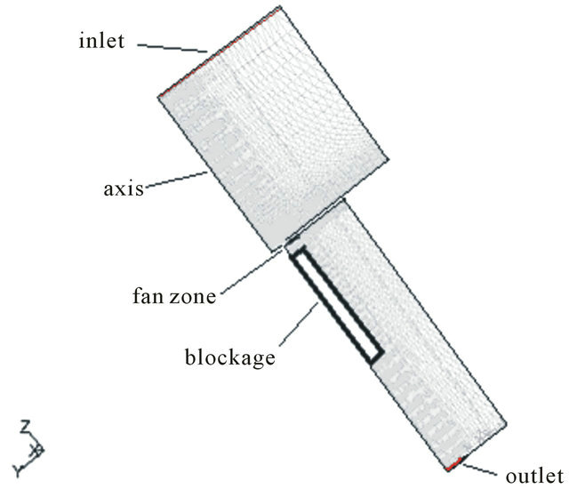
Figure 31. A meridional view of the blocked computational domain, Configuration A.
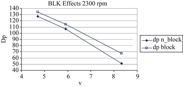
Figure 32. Effects of the block on pressure rise curves (Fan1, Configuration A, 2300 rpm) dp n block: domain without blockage dp block: domain with blockage.
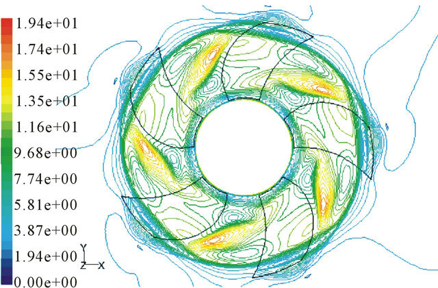
Figure 33. Velocity magnitude on a plane 5 mm downstream of the fan (domain without block, Qd, 2300 rpm).
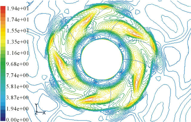
Figure 34. Velocity magnitude contours on a plane 5 mm downstream of the fan (domain with block, Qd, 2300 rpm).
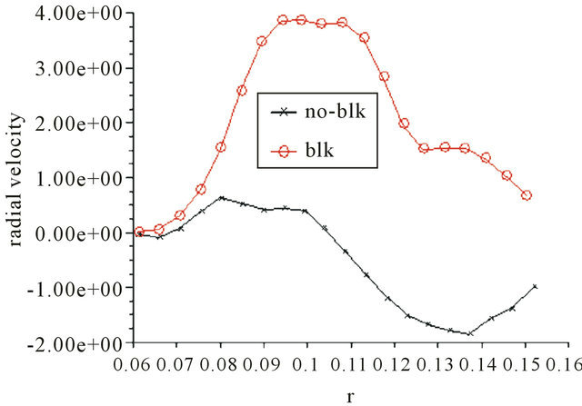
Figure 35. Averaged radial velocity on a plane 5 mm downstream of the fan (Fan1, Configuration A, Qd, 2300 rpm) no-blk: domain without block; blk: domain with block.
model suppresses the radial and tangential components of the velocity field. Since these components may be relatively large, and may be important in some applications, it is useful to discuss and compare models that ignore and models that simulate the radial and tangential velocities.
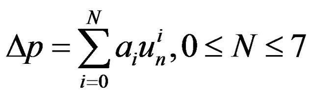
Fluent provides the user with an actuator disk type model where the fan is replaced with an infinitely thin surface (face zone) on which the pressure rise through the fan is specified by a polynomial in the normal velocity
 (1)
(1)
where  is the normal velocity component on the upstream face of the fan. If the average value of
  is used then a single value for
  is obtained, and if the local value of
  is used then a point distribution for
  is obtained. The actuator disk enforces continuity of the velocity across the fan face. In this work, this model is referred to as the “dp” model, and it is expected to work well for flows that are primarily axial, i.e., with very small radial and tangential components.
It is also possible (in Fluent) to introduce swirl velocity into the model by specifying both radial and tangential velocities on the fan face. The tangential and radial velocities are represented by polynomial functions of the form
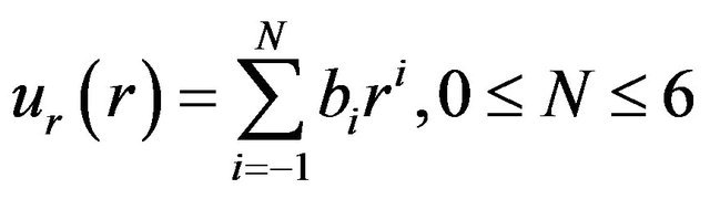 (2)
(2)
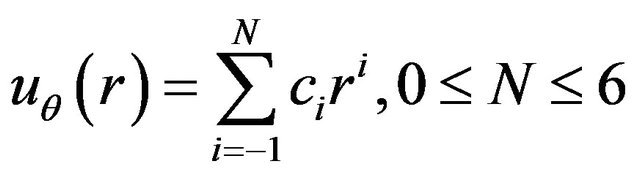 (3)
(3)
where r is the radial distance from the fan center, and  are constant coefficients obtained using the least squares method for fitting curves to data points. This model will be referred to as the polynomial (“poly1D”) model.
Neither the dp nor the poly1D models take into account any changes in the flow field that take place in the circumferential direction. The point profile fan model, which Fluent has made available, specifies the values of tangential and radial velocities at each grid point of the fan face and hence it incorporates the circumferential changes in the flow field. This model will be referred to as the profile (“prof”) model.
Another model is proposed (for the first time) in this section that also takes into account the circumferential non-uniformities of the flow velocity field, referred to as the two-dimensional (“poly2D”) model. In order to implement this model, a special source code or User Defined Function (UDF) has to be incorporated into Fluent’s code. In the UDF the radial and tangential velocity components are represented by two-dimensional polynomials in the Cartesian coordinates x-y as follows:
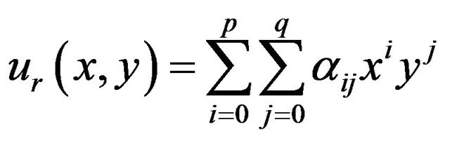 (4)
(4)
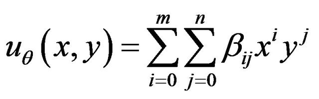 (5)
(5)
where the  and
and  are coefficients that can be obtained using any two dimensional interpolation or surface-fitting method that guarantees the required accuracy. For the simulations presented here, these coefficients are obtained using the statistical software package SAS which employs multiple regression to evaluate the coefficients.
The coefficients for the polynomial functions in the models poly1D and poly2D that represent pressure rise, radial and tangential velocities are determined using data that has been obtained from the full 3D CFD simulation of the fan (cfd model). This data could also be obtained from experimental measurements but, assuming that our full CFD calculations are accurate enough, the advantage of extracting this data from the CFD simulation is that it affords us to get the data from a plane which lies as close to the fan as we wish, certainly much closer than experiments may allow. The polynomial models are expected to perform better than the dp model because they include models for the radial and tangential velocity fields.
6.1. Effect of Using Data from Different Planes
For the poly1D model, the coefficients for the tangential and radial velocity components can be determined from curve-fitting circumferentially averaged data obtained from a plane close to the fan. One would expect that the closer this plane lies to the fan, the more accurate the results would be. This is true in general, but if this plane is too close to the fan, the results become slightly less accurate. From Table 1 it is seen that for the prediction of pressure, using data from  (i.e., 5 mm below the fan) is slightly more accurate. However, for the prediction of average velocity components on the plane lying 25 mm downstream of the fan, data from
  is slightly better for
 , but
, but  is significantly better for
  and
and .
.
The same conclusions can be drawn from examination of x-y plots of the circumferentially averaged velocity components versus radius as illustrated in Figure 36 for the tangential velocity. The loss in accuracy when using data that is obtained from the plane closest to the fan is probably due to the fact that the plane z-5 is too close to the wake of the blade, so that circumferential averaging is less reliable near the fan.
6.2. Prediction from Different Models
Pressure rise prediction from the various simplified models is in a very good agreement with the full cfd model (Figure 37). Thus, if the user is interested only in the  prediction and there is no need to include the swirl velocity components in the model, then the dp model is a good choice. On the other hand, if the details of the velocity field are important, then it is necessary to include models for
  and
and . If only circumferentially averaged values of the velocity components are needed, then
Table 1. Average values of velocity components (m/s) and pressure (Pascal) on plane 25 mm downstream of the fan (Qd = 0.299 m3/s, 2300 rpm).
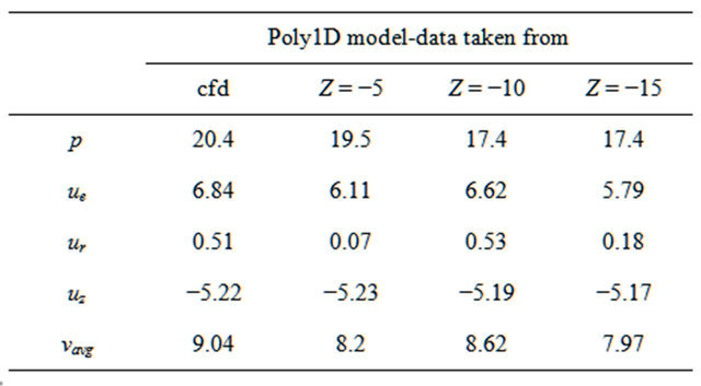
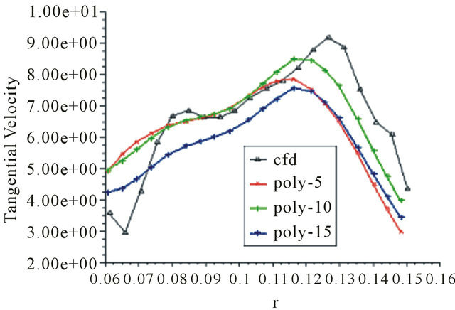
Figure 36. Comparison of predicted tangential velocities when data is taken from planes at 5, 10 and 15 mm behind the fan.
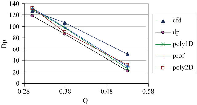
Figure 37. Static pressure rise vs flow rate: comparisons of the different models to the full cfd model, 2300 rpm.
the polynomial models perform better than the prof and dp models, as can be seen, for instance, from Figure 38 that shows radial velocity versus radius on a plane 25 mm downstream of the fan for a representative case (0.299 m3/s at 2300 rpm). In terms of convergence speed, the polynomial models are the most efficient and the dp model takes the greatest number of iterations to reach the converged state.
If the circumferential variations of the velocity field are of particular importance, then pressure and/or velocity contours must be examined. Typical contours of the velocity magnitude predicted by the various models are shown in Figures 39-42. Clearly, the prof and poly2D are in better agreement than the poly1D model. The dp model is not shown because it does not provide any reasonable prediction of the swirl velocity components. For higher flow rates, the differences between the poly1D model on one hand, and the prof and poly2D models on the other hand, become less prominent since the flow tends to mix out circumferentially.
6.3. Effects of Blockage on Models
The effects of blockage on the simplified models are investigated in this section. For that purpose, a number of
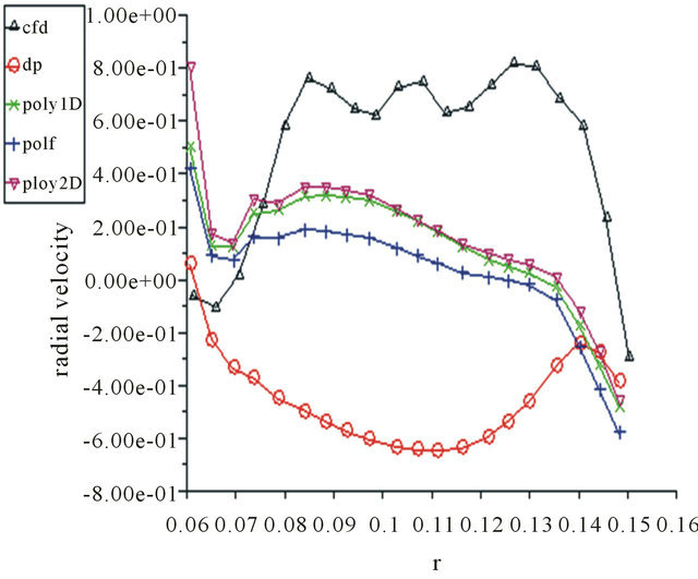
Figure 38. Comparison of various models: circumferentially averaged ur on the plane lying 25 mm downstream of the fan.
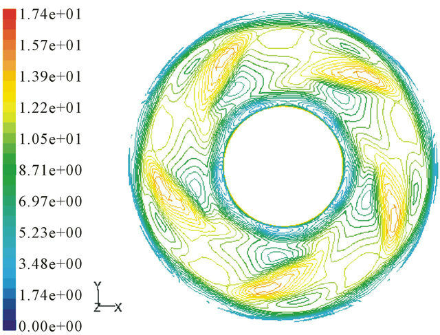
Figure 39. Contours of velocity magnitude on the 25 mm plane for the cfd model.
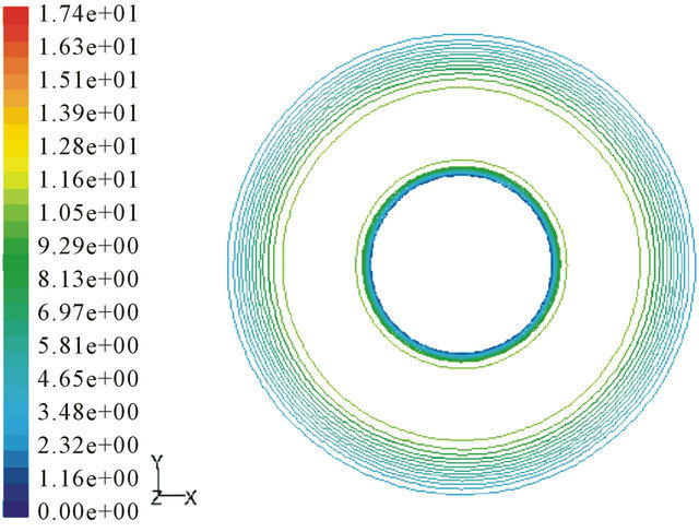
Figure 40. Contours of velocity magnitude on the 25 mm plane for the poly1D model.
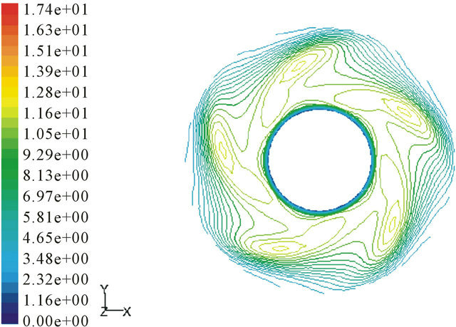
Figure 41. Contours of velocity magnitude on the 25 mm plane for the prof model.
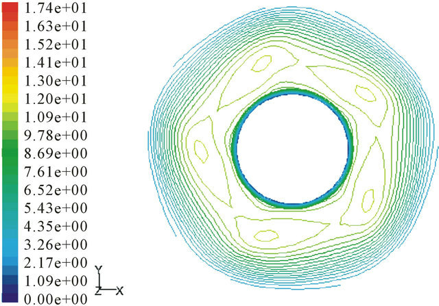
Figure 42. Contours of velocity magnitude on the 25 mm plane for the poly2D model.
numerical experiments were performed and the performances of the full CFD model with the dp model are compared.
In Figure 43 the  curves are plotted for four models, the full CFD models with and without blockage (cfd blk and cfd nblk) and the dp model, in the blockage configuration, with data for the determination of
  in Equation (6.1) taken from the cfd blk model (dp blk-data), and with data taken from the cfd nblk model (dp nblkdata).
This plot clearly demonstrates that the dp model using data from the full CFD blocked configuration simulations is significantly more accurate than if data obtained from the full CFD unblocked simulations is used. There is a good agreement between both of the dp models and the cfd model in predicting the axial velocity. Specifically, all the cases present the same radial trends for the axial velocity. The tangential and radial velocities are not predicted accurately by the dp model, but this is expected since this model completely ignores these velocity components. Surprisingly, both dp models predict almost
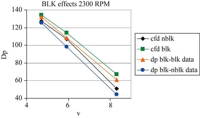
Figure 43. Static pressure rise vs velocity magnitude cfd nblk: full cfd model without blockage; cfd blk: full cfd model with blockage; dp blk-blk data: dp model with ∆p obtained from model with blockage; dp blk-nblk data: dp model with ∆p obtained from model without blockage.
identical axial velocity distribution on this plane, regardless of whether data is taken from the blocked or unblocked model. This is not true for the high flow rates since the difference in  is greatest there.
7. Conclusions
The single reference frame model of the fan is computationally efficient and captures all of the main physical features of the flow in a ducted fan. However, it is inadequate for extended mesh calculations, since the resulting unphysical Coriolis forces will dominate the all important viscous forces. Also, it does not provide a very realistic model of the fan when placed in a domain similar to that of the underhood environment. The multiple reference frame model is more suitable for such calculations.
It is possible, under most working conditions, to remove the top of the hub from the domain. Mesh generation is greatly simplified, and significant gains in terms of saving time and computer resources are achieved.
For the extended mesh calculations, it has been shown that the pressure rise and flow field can be accurately predicted by the proper implementation of the outer boundary conditions, and the location of the numerical boundary conditions can have a significant impact on the results obtained.
If the computational domain in a simplified fan model simulation involves some kind of blockage, the Dp curves and/or velocity profiles, or forces used for the implementation of the simplified fan model should be obtained from experiments or a full CFD model that also contain the same kind of blockage, because the presence of blockage downstream of the fan changes the flow significantly.
For simplified fan models, the data for the determination of the fan characteristics should be obtained from a plane as close to the fan as possible, but not too close to the fan’s wake. The dp model predicts pressure rise accurately and is recommended if the tangential and radial components of the velocity field are not important in the problem at hand. Otherwise, the profile and polynomial models would provide a more accurate representation of the details of the velocity field.
REFERENCES
- H. Capdevila and J. Pharoah, “CFD Analysis of Axial Flow Fans for Automotive Cooling Systems,” CFD95, Proceedings of the 3rd Annual Conference of the CFD Society of Canada, Banff, Vol. 1, 1995, pp. 307-314.
- E. Coggiola, B. Dessale and S. Moreau, “On the Use of CFD in the Automotive Engine Cooling Fan System Design,” AIAA-0772, 23 February 1998, pp. 1-10.
- J. Foss, D. Neal, M. Henner and S. Moreau, “Evaluating CFD Models of Axial Fans by Comparisons with PhaseAveraged Experimental Data,” Proceedings of the SAE Vehicle Thermal Management Systems Conference, Nashville, Vol. 363, 2001, pp. 83-92.
- V. Damodaran and J. Danciu, “Steady and Transient CFD Analysis of Automotive Fans,” CFD 2002, Proceedings of the 10th Annual Conference of the CFD Society of Canada, Windsor, 7-9 July 2002, pp. 360-365.
- B. A. McCormick, “Aerodynamics, Aeronautics, and Flight Mechanics,” 2nd Edition, John Wiley and Sons Inc., NY, 1995.
- W. Johnson, “Helicopter Theory,” Dover, 1994.
- J. H. W. Lee and M. D. Greenberg, “Line Momentum Source in Shallow Inviscid Fluid,” Journal of Fluid Mechanics, Vol. 145, 1984, pp. 287-304. doi:10.1017/S0022112084002937
- R. G. Rajagopalan, “Inviscid Upwind Finite Difference Model for Two-Dimensional Vertical Axis Wind Turbines,” Ph.D. Thesis, West Virginia University, Morgantown, 1984.
- R. G. Rajagopalan and C. K. Lim, “Laminar Flow Analysis of a Rotor in Hover,” Journal of the American Helicopter Society, Vol. 36, No. 1, 1991, pp. 12-23.
- W. G. Joo, “The Simulation of Turbomachinery Blade Rows in Asymmetric Flow Using Actuator Disks,” Journal of Turbomachinery, Vol. 119, No. 4, 1997, pp. 723- 732. doi:10.1115/1.2841182
- W. G. Joo, “The Application of Actuator Disks to Calculations of the Flow in Turbofan Installations,” Journal of Turbomachinery, Vol. 119, No. 4, 1997, pp. 733-741. doi:10.1115/1.2841183
- C. Leclerc and C. Masson, “Predictions of Aerodynamic Performance and Loads of HAWTs Operating in Unsteady Conditions,” AIAA-0066, Reno, 11-14 January 1998, pp. 335-345.
- C. Alinot, C. Masson and A. Smaili, “Effects of Pressure Interpolation Schemes on the Aerodynamic Simulations of Horizontal Axis Wind Turbines,” CFD 2K, Proceedings of the 8th Annual Conference of the CFD Society of Canada, Montreal, 2000.
- R. Sandboge, S. Caro, P. Ploumhans, R. Ambs, B. Schillemeit, K. Washburn and F. Shakib, “Validation of a CAA Formulation Based on Lighthill’s Analogy Using AcuSolve and Actran/LA on an Idealized Automotive HVAC Blower and on an Axial Fan,” 12th AIAA/CEAS Aeroacoustics Conference, Cambridge, 8-10 May 2006, pp. 3795-3812.
- H.-S. Chen, C.-Q. Tan, S. Kang, X.-Z. Liang, “Numerical and Experimental Study on Effects of Hub Leakage on Performance and Flow Field of Axial Fan,” Fluid Machinery, 2006, pp. 345-351.
- S. H. Liu, R. F. Huang and L. J. Chen, “Performance and Inter-Blade Flow of Axial Flow Fans with Different Blade Angles of Attack,” Journal of the Chinese Institute of Engineers, Vol. 34, No. 1, 2011, pp. 141-153.
- P. J. Nourse, “Development of an Automotive Test Facility,” MASc. Thesis, University of Windsor, Windsor, 2002.
- M. Brown, “Velocity Measurements Near an Automotive Cooling Fan,” MASc Thesis, University of Windsor, Windsor, 2001.
- H. K. Versteeg and W. Malalasekera, “An Introduction to Computational Fluid Dynamics: The Finite Volume Method,” Prentice Hall, Harlow, 1995.
- ICEM CFD Engineering, “ICEM CFD Hexa,” Manual, 1997.
- D. C. Wilcox, “Turbulence Modeling for CFD,” DCW Ind., La Canada, 1994.
- H. Schlichting, “Boundary Layer Theory,” 7th Edition, McGraw-Hill, 1979.
- J. D. Denton, “Solution of the Euler Equations for Turbomachinery Flows: Part 2, Three Dimensional Flows,” In: A. S. Ucer, P. Stow and C. Hirsch, Eds., Thermodynamics and Fluid Mechanics of Turbomachinery, NATO ASI Series, Series E: Applied Sciences—No. 97A, Vol. 1, 1985, pp. 31-47.
- FLUENT Inc., “Fluent 5, User’s Guide,” 1998.
- S. V. Patankar, “Numerical Heat Transfer and Fluid Flow,” Hemisphere, 1980.
- B. K. Shivamoggi, “Theoretical Fluid Dynamics,” John Wiley and Sons, NY, 1998. doi:10.1002/9781118032534