Applied Mathematics
Vol.4 No.1(2013), Article ID:27125,11 pages DOI:10.4236/am.2013.41007
Was There a Contagion during the Asian Crises?
1Department of Economics, Stonehill College, Easton, USA
2Department of Economics, Izmir University of Economics, Izmir, Turkey
Email: kazemi@stonehill.edu, ayla.ogus@ieu.edu.tr
Received July 29, 2012; revised November 1, 2012; accepted November 8, 2012
Keywords: Financial Crises; Contagion; Global Stock Returns and Volatility
ABSTRACT
The contagion of financial crises surrounding the markets around the world has been in the forefront of academic and public discussions. In this paper, we attempt to study the “contagion effect” of the stock market crises around the world by studying the correlations of global stock returns and volatility. We analyze the daily returns of major stock indexes around the world to discover the timing and path of the transmission of shocks that manifest themselves in stock market returns. We construct VARs of major stock market index returns and volatilities. Our work differs from the literature in analyzing spillover effects between emerging markets and other major stock markets.
1. Introduction
The contagion of financial crises surrounding the markets around the world has been in the forefront of academic and public discussions due to the experiences of Mexico in 1994, Indonesia, Japan and other Asian countries in 1997 and 1998, Russia in 1998, and Brazil in 1999. In all these cases, a number of countries experienced increased volatility and co-movement of asset prices in the aftermath of a dramatic movement in one stock market. Although greater volatility is expected during a time of financial turmoil, economists have not been able to provide a straightforward explanation for the co-movement of asset prices across countries, particularly among countries with no or very few economic links.
The transmission of increased volatility and co-movement of asset prices after financial crises has been termed contagion. There are different definitions of contagion widely used in the literature. Contagion has both been defined as increased co-movement or increased linkages across markets after shocks. The former definition is broader and refers to increased co-movement of asset prices in times of high volatility as contagion. The latter definition entails the transmission of shocks to other countries beyond any fundamental link among the countries and beyond common shocks and commonly explained by herding behavior. Contagion occurs when cross-country correlations increase during crisis times relative to correlations during stable times.
However, some economists also define contagion as the transmission of shocks to other countries. Contagion can take place both during “good” times and “bad” times and therefore does not need to be related to crises. However, contagion has been emphasized during crisis times.
Yet, some economists argue that the transmission mechanism of shocks distinguish contagion from interdependence [1]. Among economists who agree on the definition of contagion, there may be disagreement as to how to measure contagion. Linkages among markets can be measured as the correlation in asset returns of the probability of a speculative attack.
In this paper, we will define contagion as increased linkages after a shock. We provide empirical evidence for the existence of contagion during the Asian crises. We will first model the linkages among the first important stock markets and we treat these results as reflecting the economic links between countries in stable times. Next we study correlations among markets to identify cases where contagion could be said to have occurred.
We use the term “contagion effect” as the impact of the shock in one market on another market. Although each crisis can be analyzed and to some extent explained using detailed country-specific data, a possible “contagion effect” necessitates a broader perspective. Consequently, in this paper we attempt to study the “contagion effect” of the stock market crises around the world by studying the correlations of global stock returns and volatility. We analyze the daily returns of major stock indexes around the world to discover the timing and path of the transmission of shocks that manifest themselves in stock market returns. The methodology we adopt minimizes data requirements, which pose serious limitations on any empirical study that incorporates emerging markets.
We will define contagion as the increased correlation during crisis periods and suggest ways to improve on the tests performed in the empirical literature. In the next section, the related literature is discussed, followed by a detailed description of the data and methodology employed. The results pertaining to daily returns, weekly returns and volatility are discussed respectively. A summary of major findings and directions for future research conclude the paper.
2. Literature Review
There exists a body of literature that looks at correlations of stock returns across stock markets. The common approach is to look at returns on major stock market indexes in a bivariate setting and detect dependencies. Here we summarize this body of research. Reference [2] finds that international correlations are not stable over time, a finding that is also confirmed by [3,4] on monthly returns of industrial countries. In [5-7] the authors find that correlations are higher in times of high volatility and [8] finds higher correlations in more recent years. Reference [9] studies the correlations of monthly excess returns for 7 major countries over a thirty-year period and finds increased correlations between markets over time.
Our paper differs from the works mentioned above in two important ways. Firstly, our focus is the correlations between stock returns of not only industrialized countries but emerging markets as well. Secondly, we do not look at bivariate correlations as conducted in ([5,9]) but analyze the linkages across several markets simultaneously. Furthermore, we focus on shorter-term linkages, namely daily and weekly rather than monthly1. Due to data limitations posed by the emerging markets we cannot extend our analysis to monthly returns without restricting our sample of countries. In the next section, the data and the methodology we employ are described in detail.
3. Data/Methodology
Using Bloomberg Historical Data provided by Bloomberg LP, we study the daily returns on major stock indexes around the world in a theoretical vector auto-regression (VAR), which is a popular method of analyzing the dynamics of economic systems. The countries/ areas we study are the United States, the United Kingdom, Germany, Spain, Russia, Hong Kong, Singapore, Indonesia, Japan, Mexico, Argentina, Venezuela, and Brazil. The sample consists of the following indexes: S&P 500 (SPX), British Financial Times 100 Index (UKX), Spanish 35 Index, formerly FIXE 35, (IBEX), Deutsche Borse AG German Stock Index (DAX), Russian Trading System Index (RTSI$), Singapore’s Straits Times Index (STI), Hong Kong’s Hang Seng Index (HIS), Japan’s Nikkei Dow (NKY), Indonesia’s Jakarta Composite Index (JCI), Mexican Bolsa (MEXBOL), Argentina’s Stock Index (MERVAL), Venezuela’s Stock Market Index (IBVC), and Brazil’s Bovespa (IBOV). The timeframe for the analysis is constrained by the development of the Russian Trading System on September 1st, 1995.
In order to see the transmission of shocks across stock markets, we restrict lag length to 5 days. Longer lags improve forecasting ability of individual stock indexes but are costly in terms of degrees of freedom for the analysis of the system. We tested and rejected shorter lags.
We estimate the following system:
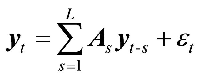 (1)
(1)
where yt is an n-vector of variables and  is an n × n matrix of coefficients. L denotes the total number of lags. εt is an n × 1 vector of errors that are uncorrelated across time, i.e.
 . Let
. Let . So in each equation there are n × L coefficients to be estimated, and in the system, there are n2L numer of coefficients.
For computing future forecasts, the ordering in the VAR is important. We order the returns on stock market indexes by time. Our reasoning is that information in the stock markets travel relatively fast, with the markets in the US, reacting to news in Japan in a matter of hours. Since the data is based on returns calculated at the close of each day, any ordering that violates the time difference in the stock markets will be missing an important component.
As mentioned earlier, we use five lags (L = 5) of each variable. Including longer lags, up to twenty lags of each variable improves forecast accuracy but at the expense of clouding dynamics among different stock markets and greatly reducing degrees of freedom. Since our primary aim in this paper is to uncover the dynamics among world stock markets, we restrict the lag length to five. We test and reject shorter lags2.
We initially started out with fourteen of the more important world stock market indexes. Block exogeneity tests suggested that we exclude MERVAL, HSI, STI, IBEX, CAC and IBVC3. Below we present the results for an eight variable VAR with SPX, UKX, DAX, NKY, MEXBOL, IBOV, RTSI$, and JCI.
4. Results
In this section, the results from the VARs based on daily returns, weekly returns and weekly volatility are discussed. First, we compute correlation coefficients in stable times and crises periods based on two-country VARs. Later, we estimate VARs for major stock market indices based on daily and weekly returns.
4.1. Correlation Coefficients
This paper deals with the question of how to measure contagion, therefore, instead of providing a list of all its possible definitions and procedures to measure it, this paper concentrates on the two most frequently asked questions raised by applied papers in this area:
First, what are the channels through which shocks are propagated from one country to another? In other words, is it the trade, macro similarities, common lender, learning, or market psychology? What determines the degree of contagion? And second, is the transmission mechanism stable over time? Or more specifically does it change during the crises?
Providing the answer to any of the previous two questions encounters important econometric limitations. Contagion has been associated with high frequency events; hence, it has been measured on stock market returns, interest rates, exchange rates, or linear combinations of them. This data is plagued with endogeneity, omitted variables, conditional and unconditional heteroskedasticity, serial correlation, non-linearity and nonnormality problems. Unfortunately, there is no procedure that can handle all these problems at the same time. And therefore, the literature has been forced to take short cuts.
We will define contagion as the increased correlation during crises periods and suggest ways to improve on the tests performed in the empirical literature. Tests are based on simple correlation coefficients in stable and crises periods.
If contagion is simply defined as increased co-movement after crises, then it is straightforward to test for contagion using correlation coefficients before and after crises. However, if we take a more restrictive approach and define contagion as increased correlation, then we need to make adjustments to our estimates of correlation coefficient because as [1] shows, the correlation coefficient is biased upwards in times of high volatility. Therefore, tests for contagion should be based on correlation coefficients adjusted for this bias.
However, the practical application of this adjustment is hampered by the low power of tests for contagion using this method. Reference [10] demonstrates the low power of tests based on heteroskedasticity adjusted correlation coefficients and shows how these tests fail to find contagion in small samples while they do when crises periods are defined to span longer periods that generate larger samples for crisis episodes. A case could be made for extending the crises periods since contagion from a crisis in one country will affect other countries with lags, different lags for different countries. Hence extending the crisis episode can be defended. However, contagion is likely to take place with shorter lags, so we may still have a problem caused by small samples for crises periods in recent and future crises.
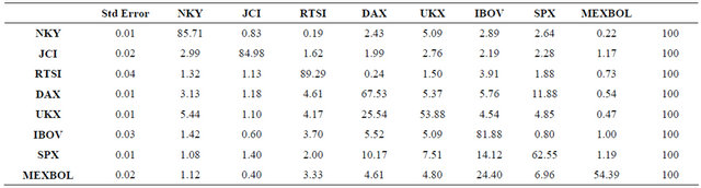
Given this evidence, how can we test for contagion? Table 1 provides the cross correlations between Hong Kong and other countries’ major stock market indexes returns. The null hypothesis is that cross correlations are greater than zero during stable times as tested in column 7 against the alternative that it is less than or equal to zero during crisis periods. The rejection of this hypothesis will constitute the evidence that the correlation coefficient is zero or less.
We also tested the null that during crisis periods correlation coefficients are less than or equal to zero. The rejection of this hypothesis is evidence that there is a positive correlation between the two markets. Therefore, rejection of the two hypotheses indicates contagion. It is not necessary to perform this test on the correlation coefficients corrected for any potential bias since if the correlation coefficient is equal to zero in stable times, it will be true that it will be also equal to zero in volatile times. The sign will also carry over. So this particular test can be performed on unadjusted correlation coefficients.
We subsequently cannot reject the null hypothesis of no or negative correlation during stable times for Taiwan, Thailand, Argentina, US and Russia. Additionally, we cannot reject the null of no or negative correlation in crisis times for Taiwan, Thailand, Mexico, US, India and South Africa. Therefore, we conclude that there was contagion from the shock to the Hong Kong stock market to the Russian market.
As Table 2 shows, if we tested the null hypothesis to prove that the correlation coefficient is negative in stable times against the alternative that it is positive, and test the null that the correlation coefficient is positive in crisis times against the alternative that it is negative, rejections of both hypotheses indicates contagion since the sign of correlation coefficient will carry over. With this test, we identify contagion from stock market shocks in Hong Kong to the Brazilian, Mexican, Indian and South African stock markets.
Based on the test results, we can also assert that there was no contagion from the Hong Kong crises to Taiwan, Thailand, Argentina and the US. The other countries have significant positive correlation in stable times and crisis times. Using the unadjusted correlation coefficients, we cannot determine whether there is contagion or not with a testing procedure that does not suffer from a low power.
We have identified contagion as the linkage among stock markets in both stable times and times of crisis.
Table 1. Test results for contagion—stable (pre-crises-period) and crises period.
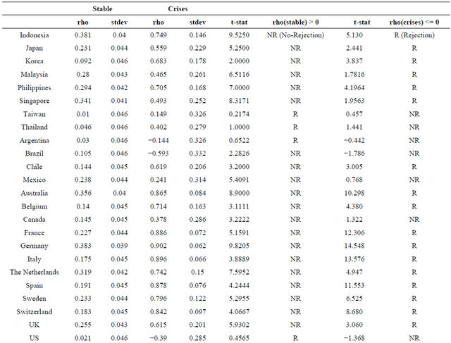

The contagion between Russia and Hong Kong is interesting since we find no linkages between the two markets during stable times but observe co-movement of their asset returns during crisis. We use a portfolio balancing argument to explain why we observe changes in linkages during crisis times. It is conceivable that countries with no linkages in their market returns during stable times to exhibit and therefore experience co-movement of their stock market returns during the more volatile times where turmoil exists.
4.2. Daily Returns
Table 3 presents the significant coefficients in each of the equations in the VAR. Each column represents one equation in the system. Significant coefficients are marked with an X. We would like to remind the reader that five lags of each variable are included in each equation. An X indicates that the coefficients for all the lags on that variable are found to be jointly significant at the 10 percent level via an F-test.
The strong interconnections between the stock markets of the industrialized world are apparent. The expected dependence of the Russian stock market on the German stock market is also reflected in the results. However, the DAX does not exhibit a similar dependence on the Russian stock market in spite the high volume of German lending to Russia.
The interdependence of the stock markets that have undergone turmoil in the recent past ISAN interesting finding. Brazilian stock market is found responsive to the Indonesian stock market but the effect seems to go only one way. The Japanese and Brazilian stock markets; The American and Indonesian stock markets exhibit strong mutual interdependence.
Table 2. Test results for contagion part ii—stable (pre-crises-period) and crises period.
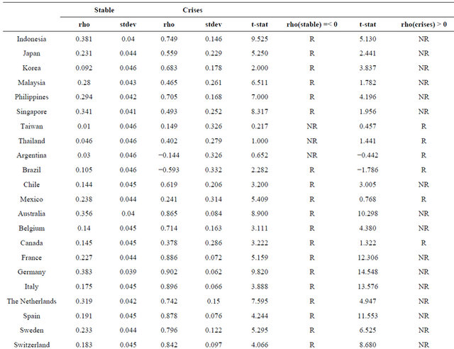
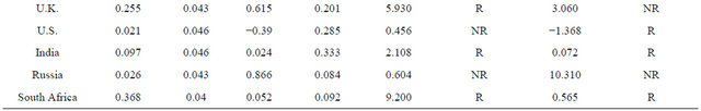
Table 3. Significant coefficients.
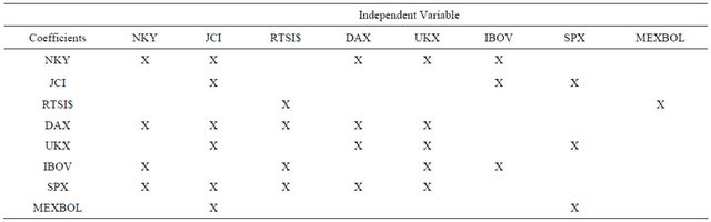
This table has implications for portfolio diversification. A shock to the NKY would have a significant effect on not only NKY, but also on JCI, DAX, UKX and IBOV since the NKY is a significant coefficient in JCI, DAX, UKX and IBOV. Suppose an investor expects the NKY to undergo a volatile period and wants to diversify away from the NKY. This in turn implies that JCI, DAX, UKX and IBOV are likely to be volatile due to the volatility in NKY. Funds should not only be diversified away from NKY but also away from these other indexes. This argument is different from a standard portfolio diversification argument that recommends the inclusion of uncorrelated stocks for diversification. Stocks may be correlated because their returns are governed by a similar set of fundamentals. A shock that affects the fundamentals would affect all the correlated stocks, but an idiosyncratic shock in one of the indexes, would not. In the context of a VAR, we can trace the effect of an idiosyncratic shock on the other indexes. In this sense, it is possible to make arguments for portfolio diversification that go beyond standard analysis.
Figure 1 represents the above information in terms of links between stock markets. If the coefficients of market A are jointly significant in explaining stock market B’s behavior and vice versa, this is represented as a two-way link between A and B. If the effect goes only one way, a one-way link in the direction of the effect will summarize the interdependence.
This figure is a useful aid for the impulse response charts in Figure 2. Impulse responses show the response of all stock markets to a one standard deviation shock in one of the markets. These shocks are orthogonalized shocks, i.e. they are shocks that only affect the stock market in question in the period that they occur. The VAR as stated in Equation (1) allows for dependence of errors in different equations. Indeed, there are global shocks that affect most if not all stock markets. Computing impulse responses for, say εt,i is not very useful if we believe that εt,i and εt,j are correlated. Impulse responses are computed for εt with the assumption that the other errors are zero which is violated in this case. The impulse responses presented are computed for idiosyncratic shocks, a shock particular to a stock market. Any shock, though as idiosyncratic as it may be, will be transmitted to other stock markets due to the interdependence that we are claiming. The impulse responses that we present show this transmission of idiosyncratic shocks, in econometric terms, shocks that are uncorrelated across equations as well as being uncorrelated across time. We use the Choleski factorization to compute orthogonolized errors4. As an example, consider the responses to a one standard deviation shock in MEXBOL. A shock in

Figure 1. Interdependence among stock markets.
MEXBOL will affect JCI and SPX. JCI will affect IBOV, SPX will affect RTSI$, NKY, DAX and UKX. The two-way link between RTSI$ and IBOV will exacerbate the initial effect before it dies out. Notice how the initial effect on JCI is large but dampens out very quickly despite the secondary effects from NKY, DAX, UKX and SPX. This is due to the low average volatility of these markets. Secondary effects from more volatile markets tend to be substantial. Both IBOV and RTSI$ are volatile indexes so the secondary effects of a shock in MEXBOL are transmitted through JCI, another volatile index, that tends to be large.
A similar story can be told of the responses to a one standard deviation positive shock to JCI. JCI affects IBOV, and through the two-way linkage between IBOV and RTSI$ which are both volatile indexes, also affects RTSI$ with one period delay. Notice that in the second period after the shock, the response in IBOV is high, compared with a very low response in RTSI$, but in the third period, the response in RTSI$ gets stronger, and remains strong until the responses die out in the seventh period.
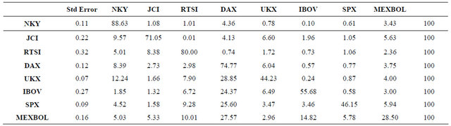
Table 4 presents the variance decompositions for the fifth period after the shock. Each row decomposes the variance of the 5-day forecast for the return one stock market index. The magnitude of the total variance is reported in the first column. Most of the variance in NKY, JCI, RTSI$ and IBOV forecasts are due to own shocks. Only the effect of shocks to UKX on NKY and IBOV are noteworthy. For the 5-day forecasts of the returns on the remaining stock markets, much if not most of the variance is again due to their own shocks. Shocks to SPX have a significant effect on forecast of DAX and to a lesser extent on MEXBOL. Shocks to DAX explain half as much of the variance due to own shocks for UKX, only matched by the effect of IBOV on MEXBOL in the
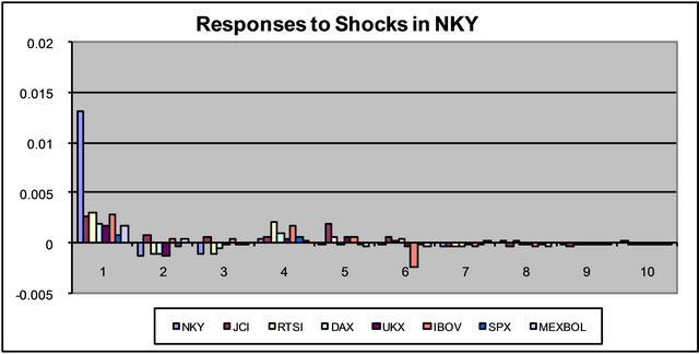
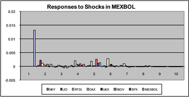
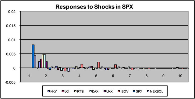


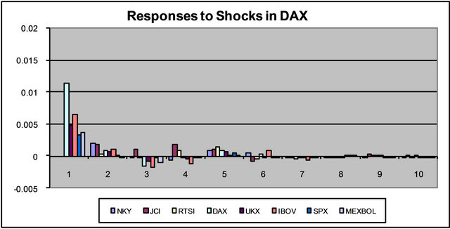
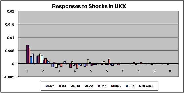
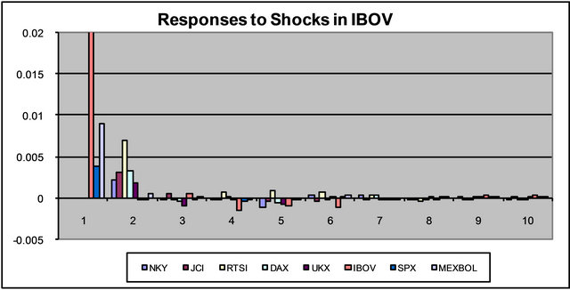
Figure 2. Impulse response functions (vertical axis) versus frequency in days (horizontal axis).
Table 4. Variance decompositions for 5-day forecasts.
system. It is surprising to note that NKY has such little effect on the other stock markets in the system. Shocks to NKY explain 5.5 percent of the variance of the 5-day forecast of UKX, but only 1 percent of the variance of the 5-day forecast in SPX. Shocks to JCI and MEXBOL have even less effect on the other markets in the system.
These numbers suggest that to get good forecasts of DAX, UKX, SPX and MEXBOL, it is necessary to include information on other variables. A good forecast of SPX, for example, requires information on IBOV, DAX and UKX.
4.3. Weekly Returns
In the previous part, daily returns are employed to estimate contagion. The advantage is, most indexes respond to shocks within a month, or even a week’s time. However, the cost of employing daily data is: confounding microstructure influences may be pretty large, including bid-ask bounce and non-synchronous trading (see reference [11] Hou and Moskowitz, 2005, RFS). To provide a more comprehensive picture, we also look at weekly returns. Following [5], we compute Thursday-to-Thursday returns and compare our results with theirs.
Table 5 presents the significant coefficients for weekly returns. Two lags of each variable are included in each equation and an X indicates that the coefficients on both lags are jointly significant at the 10 percent level.
Compared to the daily returns we see reduced interdependencies in world markets. The dependence of the Brazilian index on the Japanese index is preserved. A dependence of the British and the German indexes on the Indonesian and Russian indexes emerges.
For longer-term portfolio diversification, this table gives more hope. It exhibits less correlation across time and among global markets.
Table 6 presents the variance decompositions for the fifth period after the shock. As before, each row decomposes the variance of the 5-week forecast for the return on the stock market index. The magnitude of the total variance is reported in the first column. The indirect effects of all the markets are incorporated by the fifth week since we only include two lags in the regressions. As a result, we see a greater percentage of the variance being due to shocks in foreign stock markets.
To get good forecasts of UKX, IBOV, SPX and MEXBOL we need to include information on other variables. The NKY accounts for a substantial part of the variance of the 5-week forecast in all the other stock market returns in the system.
To compare our results with those of [5] we do not find correlations among the US and Japan, and of the US and Germany. We confirm their finding that there is no correlation between the UK and the US. When we run bivariate VARS, we also find correlations between the US and Japan, and as well as the US and Germany.
4.4. Weekly Volatility
Table 7 presents the significant coefficients for weekly returns. Two lags of each variable are included in each equation and an X indicates that the coefficients on both lags are jointly significant at the 10 percent level.
Weekly volatility seems to be transmitted among markets. Notably, volatility in the US markets is affected by volatility in the Russian, Brazilian and Mexican markets, as well as recent volatility in US markets. For emerging markets, domestic volatility overrides volatility in foreign markets. The exceptions are volatility in German markets for Brazil and Brazilian, Mexican and British markets for Indonesia.
Table 8 presents the variance decompositions for the fifth period after the shock. Each row decomposes the variance of the 5-week forecast for the return on the stock market index. The magnitude of the total variance is reported in the first column. The indirect effects of all the markets are incorporated by the fifth week since we only included two lags in the regressions.
These numbers indicate that the volatility of UKX, IBOV, SPX, and MEXBOL are endogenous to the system. It would not be possible to get good forecasts of returns on these indexes by solely relying on their past values. The NKY represents a substantial portion of the
Table 5. Significant coefficients.

Table 6. Variance decompositions for 5-week forecasts.
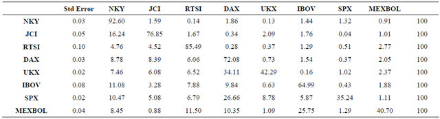
Table 7. Significant coefficients.
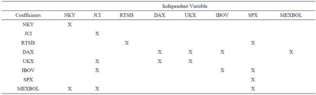
Table 8. Variance decompositions for 5-week forecasts.
forecast variance in the other stock markets. The return on DAX should be included in the forecasts of returns on UKX, IBOV, SPX, and MEXBOL, accounting for around one quarter of the 5-week forecast in each case.
5. Concluding Remarks
In this paper we studied the global transmission of stock market shocks. We analyzed the daily and weekly returns on major stock market indexes, as well as weekly volatility.
The daily returns on the Japanese stock market are impacted by daily returns on US, German, and Brazilian markets. They, in turn, influence daily returns on German, British, Brazilian and Indonesian markets. The US daily returns are found to be insensitive to daily returns on the Japanese stock market.
The daily returns on US markets are found to be moving in accordance with daily returns on Indonesian, British and Mexican stock markets. British and German daily stock returns are linked to each other, as well as those of Japan and US markets. A similar link is observed for Japan, but does not hold for the US.
Fewer dependencies are observed for Thursday-toThursday weekly returns. German and British weekly returns are influenced by weekly returns on Indonesian and Russian markets; Brazilian weekly returns are dependent on Japanese daily returns. These results demonstrate that emerging market returns influence returns on other stock markets, i.e. correlations between emerging and established market returns may be more important than correlations between major global stock market returns. Emerging markets are prone to large shocks, whose repercussions can be observed in other established markets.
In our study we also look at the transmission of weekly volatility. We measure volatility with the annualized standard deviation of weekly returns. Our results show that volatility in German and British markets have as wide repercussions as volatility in emerging markets. In general, linkages in daily or weekly returns are not preserved. The US market returns do not move together with daily or weekly returns in other markets but US market volatility is linked to volatility in the more volatile markets.
REFERENCES
- K. Forbes and R. Rigobon, “No Contagion, Only Interdependence: Measuring Stock Market Co-Movements,” Journal of Finance, Vol. 57, No. 5, 2000, pp. 2223-2261.
- P. Bennett and J. Kelleher, “The International Transmission of Stock Price Disruption in October 1987,” Federal Reserve Bank of NY Q. Review, Vol. 13, No. 2, 1988, pp. 17-33.
- M. King, E. Sentana and S. Wadhwani, “Volatility and Links between National Stock Markets,” Econometrica, Vol. 62, No. 4, 1994, pp. 901-934. doi:10.2307/2951737
- E. Kaplanis, “Stability and Forecasting of the Co-Movement Measures of International Stock Market Return,” Journal of International Money & Finance, Vol. 7, No. 1, 1988, pp. 63-75. doi:10.1016/0261-5606(88)90006-X
- L. Ramchand and R. Susmel, “Volatility and Cross CorRelation across Major Stock Markets,” Journal of Empirical Finance, Vol. 5, No. 4, 1998, pp. 397-416. doi:10.1016/S0927-5398(98)00003-6
- M. King and S. Wadhwani, “Transmission of Volatility between Stock Markets,” Review of Financial Studies, Vol. 3, No. 1, 1990, pp. 5-33. doi:10.1093/rfs/3.1.5
- E. Bertero and C. Mayer, “Structure and Performance: Global Interdependence of Stock Markets around the Crash of October 1987,” Center for Economic Policy Research, Discussion Paper, No. 307, 1989.
- P. D. Koch and T. W. Koch, “Evolution in Dynamic Linkages across National Stock Indexes,” Journal of International Money & Finance, Vol. 10, No. 2, 1990, pp. 231- 251. doi:10.1016/0261-5606(91)90037-K
- F. Longin and B. Solnik, “Is the Correlation in International Equity Returns Constant: 1960-1990?” Journal of International Money & Finance, Vol. 14, No. 1, 1995, pp. 3-23. doi:10.1016/0261-5606(94)00001-H
- D. Zhumabekova and D. Dungey, “Factor Analysis of a Model of Stock Market Returns Using Simulation-Based Estimation Techniques,” Pacific Basin Working Paper Series 01-08, Federal Reserve Bank of San Francisco, San Francisco, 2001.
- K. Hou and T. Moskowitz, “Market Frictions, Price Delay, and the Cross-Section of Expected Returns,” Review of Financial Studies, Vol. 18, No. 3, 2005, pp. 981-1020. doi:10.1093/rfs/hhi023
NOTES
1All the works we cite except for [5] are based on monthly returns and volatility. [5] study Thursday-to-Thursday weekly returns.
2This is done via likelihood ratio tests. Two VARs with different lags are estimated and their log likelihood values are compared with suitably correcting for sample size.
3See footnote 2 above.
4A lower triangular matrix G that is the solution to GG’ = Ω is computed and vt = utG−1 are used as the new shocks.