Journal of Environmental Protection
Vol. 3 No. 12 (2012) , Article ID: 26017 , 18 pages DOI:10.4236/jep.2012.312183
A Tool for Public PM2.5-Concentration Advisory Based on Mobile Measurements
![]()
Department of Atmospheric Sciences, Geophysical Institute and College of Natural Science and Mathematics, University of Alaska Fairbanks, Fairbanks, USA.
Email: *molders@gi.alaska.edu
Received September 11th, 2012; revised October 5th, 2012; accepted November 7th, 2012
Keywords: WRF; CMAQ; PM2.5; Air Quality; Interpolation; Arctic
ABSTRACT
A tool was developed that interpolates mobile measurements of PM2.5-concentrations into unmonitored areas of the Fairbanks nonattainment area for public air-quality advisory. The tool uses simulations with the Alaska adapted version of the Weather Research and Forecasting (WRF) and the Community Modeling and Analysis Quality (CMAQ) modeling system as a database. The tool uses the GPS-data of the vehicle’s route, and the database to determine linear regression equations for the relationships between the PM2.5-concentrations at the locations on the route and those outside the route. Once the interpolation equations are determined, the tool uses the mobile measurements as input into these equations that interpolate the measurements into the unmonitored neighborhoods. An episode of winter 2009/10 served as database for the tool’s interpolation algorithm. An independent episode of winter 2010/11 served to demonstrate and evaluate the performance of the tool. The evaluation showed that the tool well reproduced the spatial distribution of the observed as well as simulated concentrations. It is demonstrated that the tool does not require a database that contains data of the episode for which the interpolation is to be made. Potential challenges in applying this tools and its transferability are discussed critically.
1. Introduction
As observations indicated that concentrations of particulate matter with diameter than 2.5 µm (PM2.5) exceeded the Environmental Protection Agency 24-hour National Ambient Air Quality standard (NAAQS) of 35 µg/m3 periodically in Fairbanks, Alaska during the past years [1], Fairbanks was assigned a PM2.5-nonattainment area. In winter 2008/09, the Fairbanks North Star Borough started measuring PM2.5-concentrations along roads in commercial and residential areas with instrumented vehicles (called sniffer hereafter) (Figure 1) to obtain a broad picture of the PM2.5-concentration distribution within the nonattainment area and for public air-quality advisory. For public advisory, however, it is desirable to show spatial distributions rather than data along the vehicle routes. Such spatial distributions require intelligent interpolation.
Various studies investigated the accuracy of procedures applied to interpolate concentrations of chemically reactive gases and particles into space. One study [2], for instance, used data of ozone and particulate matter with aerodynamic diameter less than 10 µm (PM10) from sta-
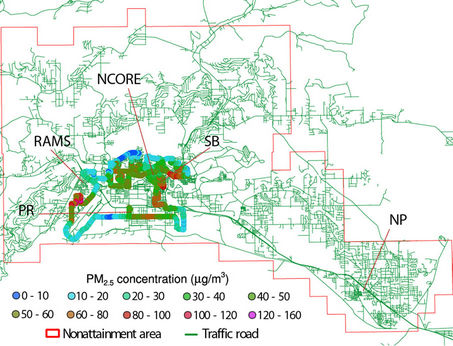
Figure 1. PM2.5-concentrations as measured in Fairbanks by the sniffer (lines of dots) on 01-02-2010 during the drive starting at 1404AST with the street network superimposed. The locations of the SB, RAMS, PR, NP, and NCORE stationary PM2.5-observation are indicated.
tionary monitoring sites and left out data from one site to compare the spatial averaging, nearest neighbor, inverse distance weight and the kriging interpolation methods. This cross-validation suggested that all tested interpolation methods performed reasonably well and the kriging method provided the least biases. Application of the universal kriging procedure for spatial interpolation of ozone data from ten monitoring stations to all zip-code areas in Atlanta, Georgia showed that over 1993 to 1995, the ozone distribution highly correlated with the wind fields [3]. This study also suggested that the Atlanta ozone-nonattainment area would expand from 56% under the 1 h ozone-standard to 88% under the 8 h ozone-standard of the Atlanta metropolitan statistical area.
While many studies apply these traditional interpolation methods in areas of sufficient data density, these methods may be problematic in areas of sparse data density [4]. The distribution of air pollutants namely is a function of many factors such as atmospheric conditions, land-use, sources (e.g. emissions, chemical reactions) and sinks (e.g. chemical reactions, deposition) [5]. These factors can vary substantially in space and time. Thus, interpolating data from sparse monitoring networks based alone on statistics of observations may provide inadequate results [4]. Therefore, first efforts were made to develop procedures that add other information to provide interpolated values. Fuentes and Raftery [6], for instance, suggested to combine observations from the Clean Air Status and Trends Network with output from an air-quality model in a Bayesian way to obtain a high-resolution sulfur dioxide distribution over the US for model evaluation. Their interpolation approach incorporated information on the emissions and underlying driving physical and chemical processes.
In this study, we present a tool to interpolate mobile measurements of PM2.5-concentrations over the Fairbanks nonattainment area. We developed this tool by combining the output from the Weather Research and Forecasting (WRF; [7]) and the Community Modeling and Analysis Quality (CMAQ; [8]) modeling systems in its Alaska adapted version [9] as a database to determine the equations needed to interpolate the mobile PM2.5-concentration observations into unmonitored neighborhoods. The tool is to provide spatial distributions of PM2.5-concentrations for public air-quality advice.
2. Simulations
2.1. Model Setup
The meteorological conditions were simulated by WRF version 3.2 in forecast mode using three nested domains (Figure 2; [10]). The outermost domain (domain 1) encompasses Alaska, and parts of Siberia, the North Pacific and Arctic Ocean with 400 × 300 grid-cells of 12 km increment. Domain 2 covers Interior Alaska with 201 × 201 grid-cells of 4 km increment. The inner most domain (domain 3) encompasses the nonattainment area and western part of the Fairbanks North Star Borough with 201 × 201 grid-cells of 1.3 km increment. The simulations were performed concurrently on all three domains in one-way coupled mode. This means the boundary conditions for each child domain stem from its parent domain, but the child domain does not feedback to the simulation of the parent domain. The physical options (Table 1) were chosen based on the experience from previous modeling studies over Alaska for winter [10,18,19].
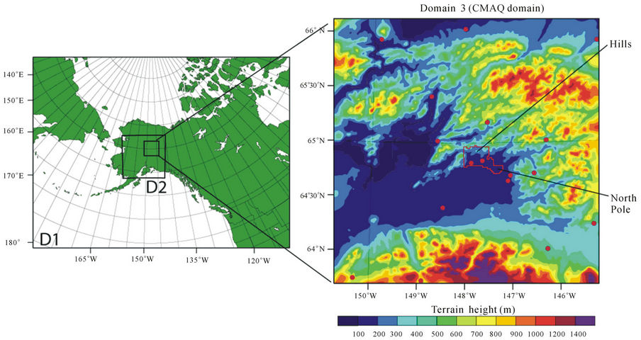
Figure 2. Schematic view of the domains used in the WRF—(left) and CMAQ simulation domains. On domain 3, terrain height is superimposed (right). Red circles indicate the surface meteorological sites used in the evaluation. The red polygon marks the Fairbanks PM2.5-nonattainment area.
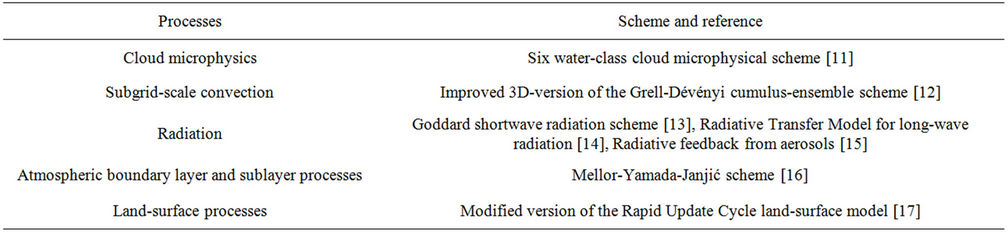
Table 1. Parameterizations used in the WRF simulations.
The CMAQ-simulations were performed and driven by the WRF-simulated meteorology of domain 3. We used CMAQ in its Alaska adapted version [9]. Parameters needed by CMAQ, but not provided by WRF were diagnosed by the Meteorology-Chemistry Interface Processor [20] with the modifications given in [9]. Gas-phase chemistry was treated in CMAQ by the Carbon-Bond mechanism [21]. Aerosol chemistry was calculated by the fifth-generation CMAQ-aerosol model [22]. Aqueous chemistry was treated following the so-called RADM mechanism [23]. The treatment of secondary organic aerosol chemistry and physics was based on the so-called SORGAM [24] with the modifications of the gas-phase chemistry fields and saturation concentrations for aromatics, terpenes, alkanes and cresols as documented by Buyn et al. [20]. Horizontal and vertical advections were calculated using the global mass-conserving scheme [25]. Horizontal diffusion was determined based on diffusion coefficients derived from local wind deformation [8]. Vertical diffusion was calculated using the K-theory approach [9,26].
We used the modifications tested and implemented for Alaska conditions [9]. The modifications include slightly lower minimum and maximum thresholds for the eddy diffusivity coefficients and a reduction of the minimum mixing height from 50 m to 16 m as observed in Fairbanks. Dry deposition of aerosols and gases was treated according to the standard procedure in CMAQ [20], but was enlarged for dry deposition on snow and Alaska-specific vegetation [27] and onto the various types of tundra [9].
2.2. Emission Inventory
Anthropogenic emissions stem from the first version of the Fairbanks 2008 emission inventory provided by Sierra Research Inc. [2011; pers. comm.]. To apply this emission inventory to winter 2009/2010 and winter 2010/2011, we assumed an emission increase of 1.5%/ year in accord with other studies [27,28]. The Sparse Matrix Operator Kernel Emissions Model [29,30] served to allocate these “updated” emissions onto the CMAQdomain in time and space based on the information on emission-source activities, land-use and population density within each grid-cell.
Anthropogenic emissions include emissions from point sources, area sources, traffic and non-road traffic. We applied a temperature-adjustment factor to the temporal allocations of the anthropogenic emissions. Herein, emissions will be higher (lower) on days having daily mean temperatures below (above) the 1970-1999 monthly mean temperature [28,31].
2.3. Simulations
The meteorological initial and boundary conditions for domain 1 were downscaled from the 1 × 1, 6 h-resolution National Centers for Environmental Prediction global final analyses. The meteorology was initialized every five days. Alaska typical background concentrations served as initial condition for the chemical fields [9]. Note that various studies [28,32,33] showed hardly any advection of PM2.5 of notable concentrations (>2 µg/m3) into Interior Alaska. To spin up the chemical fields we started the simulation three days prior to the period of interest. The chemical fields at the end of a simulation served as the initial conditions for the simulation of the next day.
We performed simulations for two episodes that had mobile measurements and occasional PM2.5-concentrations above the NAAQS at the official monitoring site at the State Office Building or other sites. We used episode 1 (December 27, 2009 to January 11, 2010) to build the database needed by the tool that we developed. We used episode 2 (January 1 to 30, 2011) for evaluation of the developed tool. Not every day of these episodes had sniffer measurements. In total, there were 13 and 14 sniffer drives with 49 h and 30 h of data during episodes 1 and 2, respectively.
2.4. Model Evaluation
Meteorological surface observations were available at 14 and 18 sites for episodes 1 and 2, respectively, from the Western Regional Climate Center and the National Climate Data Center (Figure 2).
PM2.5-observations were available at the State Office Building (SB), Peger Road (PR), Pioneer Road
(NCORE), in the community of North Pole (NP), and at the Relocatable Air Monitoring System (RAMS) trailer locations (Figure 1). Hourly observations of total PM2.5-mass measured by Met-One Beta Attenuation Monitors were available at the SB (called SB_BAM hereafter) and the RAMS (RAMS_BAM). Filter based 24h-average PM2.5-concentrations using the Federal Reference Method were available at the SB (called SB_FRM hereafter), RAMS (RAMS_FRM), NP, PR and NCORE on a 1-in-3-days basis. The SB and NCORE sites are located in commercial-residential areas whereas the PR and NP-sites are located in mixed industrial-residential areas. During episodes 1 and 2, the RAMS was located in a residential area. During episode 2, the RAMS was located about 1.5 km north of its location during episode 1. Since there had been repeatedly technical problems with the RAMS during episode 2 [Conner 2009; pers. comm.], we excluded the RAMS-observations from the evaluation of episode 2.
We calculated performance skill-scores [34] to evaluate the WRF-performance with respect to simulating meteorological quantities. These skill scores include the mean bias, root-mean-square error (RMSE), standard deviation of error (SDE), and the correlation coefficient (R).
We evaluated the simulated PM2.5-concentrations by the fractional bias
 fractional error
 normalized mean bias
 normalized means error
 mean fractional bias
 and mean fractional error

[35,36]. Here N is the number of pairs of simulated (CS) and observed (CS) PM2.5-concentrations. In addition, we determined the percentage of pairs of simulated and observed PM2.5-concentrations that agreed within a factor of two (FAC2). The correlation-skill score R between simulated and observed quantities was tested for its statistical significant using t-tests at the 95% confidence level.
3. Tool Development
3.1. Mobile Measurements
The mobile measurements encompass GPS-coordinates, PM2.5-concentrations and ambient air temperature recorded every 2 seconds while the vehicle traveled at up to 48 km/h. We performed a quality assurance/quality control (QA/QC; for details see [28]) on all mobile measurements. This QA/QC discarded all temperature and PM2.5-data for which the measured temperature deviated more than the 1971-2000 monthly-mean diurnal temperature range from the mean temperature determined from all temperature-data of the respective drive. This QA/QC ensured to discard data taken when the vehicle pulled out and the sensors were still adjusting to the outside air. The QA/QC-procedure also discarded all PM2.5-concentrations that differed >5 μg/m3 between two consecutive measurements to avoid errors from plumes from buses or trucks that emit at about the sniffer height (~2.44 m) and may have hit the sniffer.
We developed the interpolation tool using the output of the CMAQ simulations of the first episode as a “grand truth” as there was no special field campaign that provided high spatial resolution measurements in the nonattainment area. Thus, the spatial resolution of the interpolated mobile measurements is 1.3 km, i.e. the same as the CMAQ-simulation. The tool requires a database of PM2.5- concentrations simulated by CMAQ or any other airquality model. In this study, we used PM2.5-concentrations simulated by CMAQ in episode 1 as the database. This database is called CMAQ-database hereafter. It has 2592 PM2.5-concentrations at each of the 395 grid-cells in the nonattainment area, i.e. 1,023,840 data in total.
As is demonstrated later, the database does not require air-quality model simulations of the episode for which measurements are to be interpolated. The database just needs to cover the range of measurements and ideally should represent similar conditions. The advantage of this concept is that users do not have to run an air-quality model each time when they want to interpolate mobile measurements.
The CMAQ-database serves to establish the linear-regression of the PM2.5-concentration at the grid-cell, for which a concentration has to be interpolated, with the PM2.5-concentrations at the grid-cells traveled by the sniffer. These linear-regression equations—called interpolation equations hereafter—base on simulated data only. Thus, the tool permits to provide these relationships for any travelled route. This means the tool does not become useless when new roads are constructed or the vehicle is detoured.
The basic operational concept of the tool, data flow and technical steps are schematically viewed in Figure 3.
Figure 3. Schematic view of the data flow and procedure of the development of the interpolation equations.
Once measurements are taken, the above mentioned QA/QC is performed (see [28] for details). The QA/QC approved PM2.5-measurements are projected onto the grid using the GPS-data. Then the tool averages over all QA/QC approved observations that were taken in the same grid-cell and hour. Note that smaller time intervals are possible when the database is established at a smaller time step than one hour. This averaging leads to one value per hour for each grid-cell on the route during that hour. These averaged concentrations are called “observed concentrations” hereafter.
To develop the interpolation equations the tool determines the route based on the GPS data of the drive. In this step of deriving the interpolation equations, the tool uses the CMAQ-database (Figure 3). An interpolation equation is determined for each grid-cell i that is not on the route
 (1)
(1)
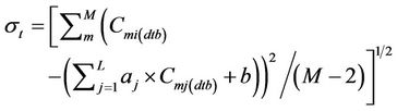
Here CMi(dtb) are the concentrations form the database in the neighborhood at the grid-cell i for which the interpolation is to be done. Furthermore, CMj(dtb) are the concentrations  in the database at the N grid-cells on the route, and aj and b are the linear-regression coefficients, respectively. Furthermore, M is the number of data for each grid-cell in the CMAQ-database. Recall that this database was obtained from the CMAQ-simulations on a 1-in-10-minutes basis at each grid-cell. Thus, when using episode 1 as database M = 2592 at each grid-cell. The determination of the interpolation Equation (1) leads to the coefficients aj and b based on least-square linear-regression.
Once the tool has determines the coefficients aj and b using the database, we have for each grid-cell one equation of the type
 (2)
(2)
At the start of the algorithm development, by using the CMAQ-database the tool considers all the concentrations at all N grid-cells on the route in determining the aj and b coefficients. In the next step, it determines an adjusted determination coefficient
 (3)
(3)
to assess the accuracy of Equation (2). In Equation (3),  is the mean of the M concentrations at i from the database. Note that so far only the GPS-observations are used to determine the route and to derive the coefficients aj and b using the database.
As suggested by Equation (3), the closer  is to 1, the lower is the interpolation error. The magnitude of
  increases (decreases) when those concentrations
  on the route
  available in the CMAQ-database are excluded (included) in Equation (1) that are unimportant in describing
 . Consequently, not all concentrations available in the CMAQ-database along the route are required to interpolate the concentration at a grid-cell i in the neighborhood outside the route.
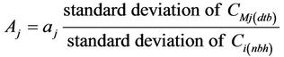
Thus, to optimize the accuracy of Equation (2), the tool now determines which grid-cells along the route can be excluded from building Equation (2). In doing so, the tool calculates the standardized regression coefficient
 (4)
(4)
This coefficient indicates the importance of the concentrations  at the grid-cell i on the route in determining the concentrations
 at grid-cell i outside the route. The tool then excludes the concentrations
  at a grid-cell j on the route for which Aj is lowest. Then it re-determines the aj and b-coefficients with the concentrations
  at the remaining L grid-cells on the route again. In doing so it again uses the concentrations from the CMAQ-database. Note that L is the number of remaining grid-cells on the route deemed important so far. The tool repeats the procedure until the obtained
  reaches a maximum. After this step, the final coefficients aj and b and final form of Equation (2) are established leading to the interpolation procedure
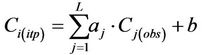 (5)
(5)
Here  is the concentration to be interpolated at grid-cell i, and Cj(obs) are the observed concentrations at the L grid-cells on the route.
Now the tool takes the observed concentrations  as the input into the optimized Equation (5). Recall that such optimized equations exist for each grid-cell i, for which an interpolation is to be done. Furthermore, L can be as large as N and differs among grid-cells for which the interpolation is to be done. The reason why L is different for different grid-cells is that for each grid-cell i, a different number of grid-cells and different grid-cells on the route may be important for the concentration at i. Thus, for each grid-cell i by using the optimized Equation (5) the tool now interpolates the concentrations
  at grid-cell i that is in the neighborhood, i.e. outside the route.
In theory, the aj and b-coefficients can be either positive or negative. Therefore, theoretically, Equation (5) could predict  if the observed concentration
  differs strongly from the concentrations in the CMAQ-database
  at one or more grid-cells of the route. In such case, the tool applies an extra treatment to satisfy the non-negative constrain of
  (Figure 3). The tool applies an analogous procedure as it does when identifying which grid-cells in the CMAQdatabase are important to describe the concentration at grid-cell i when optimizing the accuracy of Equation (5). However, in the extra treatment, instead of including
  in all L grid-cells on the route, Equation (5) only includes those in the K grid-cells for which the standardized regression coefficients obtained from Equation (4) are in descending order
 .
.
Here, K is the number of the remaining grid-cells included in Equation (5), for which Equation (5) interpolates the lowest . This means the tool only considers
 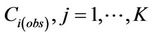 at grid-cells on the route that are most important to interpolate
 .
.
The tool then assesses the uncertainty of the interpolation. We determined the confidential interval CI, i.e. the uncertainty at the 95% level of confidence for interpolating  from
from  as [37,38]
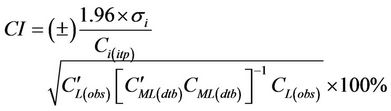 (6)
(6)
Note that when the above-described extra treatment had to be applied L has to be substituted by K in Equation (6). In Equation (6),  and
and  are the transposed matrixes of
  and
and  which are expressed as a matrix of the M concentrations at the L grid-cells on the route as:
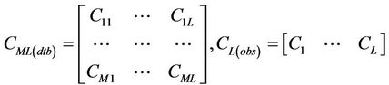 Furthermore,
The uncertainty  increases as the difference between the observed concentration
  and the concentration in the CMAQ-database
  increases.
All the above means that there is no unique set of interpolation equations tied for all potential routes in the nonattainment area. Instead, the tool develops self-consistently a set of interpolation equations for each desired route.
Our tool automatically applies the above procedure and determines an optimized interpolation equation set for the grid-cells for which the interpolations are to be done. The design of our tool allows any route within the nonattainment area. Therefore, it provides high flexibility for future mobile measurements and will be still usable after new road construction. Its design also guarantees that the tool can be transferred easily to other regions. The only pre-requisite is that a sufficient large dataset of air-quality model data is established for that region.
3.2. Sensitivity Studies
To assess how large the database has to be, we performed various sensitivity studies with reduced database sizes. These studies showed that a reduction of the database by 30% reduces the interpolation accuracy by 10%.
Wind-patterns and temperatures affect the PM2.5-distribution over the nonattainment area [1]. Therefore, we examined whether the accuracy of the tool would increase when the tool considered information on wind-direction, wind-speed or temperature. We developed an interpolation equation like Equation (5) for eight wind-direction sectors of 45˚ width. Analogously, we developed interpolation equations like Equation (5) for wind-speeds below 1 m/s, between 1 and 2 m/s, and above 2 m/s, and for temperatures below −20˚C, between −20˚C and −10˚C, and above −10˚C.
Since the objective of the tool is to provide public spatially differentiated air-quality advice, wind data must be accessible when a drive is completed. The meteorologycal tower located in downtown Fairbanks is the only site that fulfills this criterion. Temperature data are available directly from the sniffer measurements. Temperature was processed in analogous way as PM2.5-concentrations [28] to obtain observed temperature at the resolution of the interpolation grid. These observed temperatures then were included in developing Equation (5). The inclusion of any of the meteorological quantities means a reduction of the CMAQ-database to only those concentrations that were determined for the respective meteorological conditions. For instance, there were only 264 concentrations in the CMAQ-database when the simulated wind-direction at the meteorological tower fell between 0 and 22.5 degrees.
In including wind-direction, we used those concentrations in the database for which the WRF-derived wind directions fell in the same wind-direction category that was observed at the meteorological tower during the mobile measurements. We evaluated the accuracy of the wind-direction sensitive interpolation algorithm with the CMAQ-simulated PM2.5-concentrations of episode 2. Recall that the CMAQ-database based on CMAQ-simulations of episode 1. Consequently, the data used for evaluation and development are independent. We compared the interpolated PM2.5-concentration distributions obtained with and without wind-direction-consideration and their accuracy. We repeated the above steps for consideration of wind-speed and for consideration of temperature.
These sensitivity studies showed that the development of Equation (5) without considering any meteorological quantities provided best accuracy (see discussion for details). Therefore, the following discussion of the tool evaluation is for the tool without consideration of meteorological quantities in the interpolation procedure.
3.3. Tool Evaluation
We evaluated the interpolation performance by examining the FB, FE, NMB, NME, FAC2 and R using three different methods. We evaluated the interpolated PM2.5- concentrations with the PM2.5-concentrations observed at the SB_BAM and NP_BAM and RAMS_BAM sites where hourly PM2.5-observations were available for episodes 1 and 2.
In addition, we used the cross-validation method [2] to evaluate the accuracy of the developed interpolation algorithm. This method leaves out measurements in gridcells on the route sequentially. The tool then interpolates the PM2.5-concentrations by using just the remaining measurements. The left-out measurements are used for evaluation of the interpolation accuracy. The cross-validation method was applied for sniffer measurements in episodes 1 and 2.
Since the cross-validation method can only be applied to grid-cells that are on the route, we applied a method similar to PaiMazumder and Mölders [4] to further assess the tool’s accuracy. In doing so, we considered the CMAQ-simulated PM2.5-concentrations of episode 2 as the “grand truth”, i.e. we assumed that these concentrations represent the actual situation on any given day during episode 2. We used the GPS-data of routes performed during episode 2, and pulled the PM2.5-concentrations simulated for episode 2 at the grid-cells on those routes as “measurements”. By using the CMAQ-database and the GPS-observations, the tool developed the interpolation equations along the routes of episode 2. We applied the so determined interpolation equations to interpolate the concentrations from the “measurements” along the routes into the neighborhoods. We then evaluated the interpolated with the “grand truth” PM2.5-concentrations.
4. Results and Discussion
4.1. Evaluation of Simulated Meteorology
WRF performed relatively similar in predicting the meteorological quantities of episodes 1 and 2 (Table 2). WRF well captured the temporal evolutions of 2m temperature and 2 m dew-point temperature, 10 m wind-speed and sea-level pressure. Throughout both episodes, WRF consistently predicted warmer and drier near-surface conditions, and stronger 10m wind-speeds than observed (Figure 4, Table 2). The overestimation of wind-speed under weak wind conditions (v < 1.5 m/s) like during our episodes is common to all modern meteorological models [27,28,39,40].
WRF well captured the temporal evolution and magnitude of sea-level pressure. On average, WRF predicted much drier (27% lower in relative humidity) conditions than observed especially between January 8 and 10, 2011 (Figure 4). WRF simulated wind-direction with a mean bias < 30˚, i.e. this performance falls within the range of other models for this region [27,28,41-43]. WRF generally underestimated downward shortwave radiation throughout episode 1 by 33 W/m2, on average. In episode 2, WRF underestimated downward shortwave radiation for January 1 to 10, 2011 by 63 W/m2 on average, while it overestimated downward shortwave radiation on the other days by 97 W/m2 on average.
4.2. Evaluation of CMAQ Simulated PM2.5-Concentrations
The evaluation with measurements at fixed sites showed
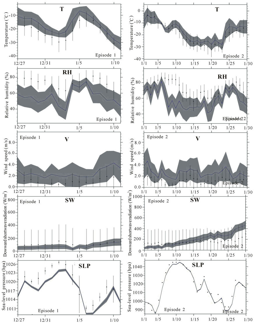
Figure 4. Temporal evolution of daily averaged 2 m temperatures (T), wind-speed (v), relative humidity (RH), accumulated downward shortwave radiation (SW), and sea-level pressure (SLP) averaged over the 14 and 18 sites for which observations were available during episodes 1 and 2, respectively. The solid blue line and closed circles indicate simulated and observed quantities; grey-shading and vertical bars indicate the variance of the simulated and observed quantities, respectively.
that CMAQ performed relatively better in predicting PM2.5-concentrations for episode 1 than for episode 2 (Table 3). Over all sites and days, the mean bias, RMSE, NMB, NME, and FAC2 of 24 h-average PM2.5-concentrations for episode 1 are 4.4 µg/m3, 28.8 µg/m3, 9%, 42% and 91%, respectively. The corresponding values for episode 2 are 31.7 µg/m3, 44.1 µg/m3, 125%, 129% and 49%. Typically, air-quality model simulations that have FB within ±30% and a FAC2 ≥ 50% are considered as having good performance [35]. Typically, MFB
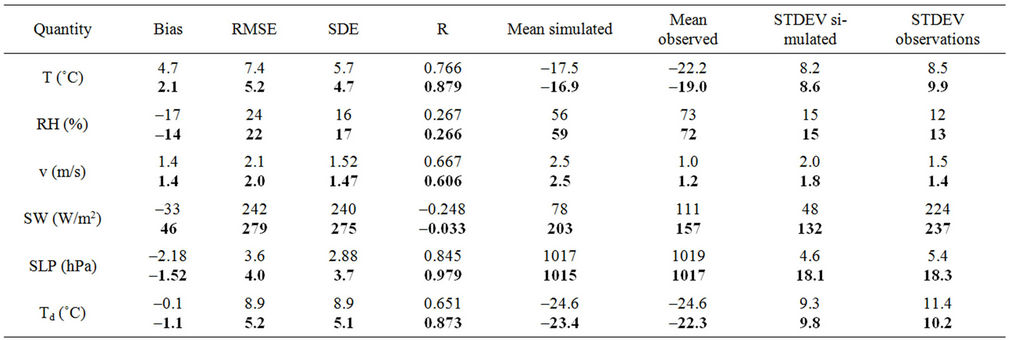
Table 2. Performance skill-scores of WRF in predicting 2 m temperature (T), 2 m relative humidity (RH), 10 m wind-speed (v), accumulated downward shortwave radiation (SW), sea-level pressure (SLP), and 2 m dew-point temperature (Td) in episode 1 (normal print) and episode 2 (in bold). STDEV is the standard deviation.
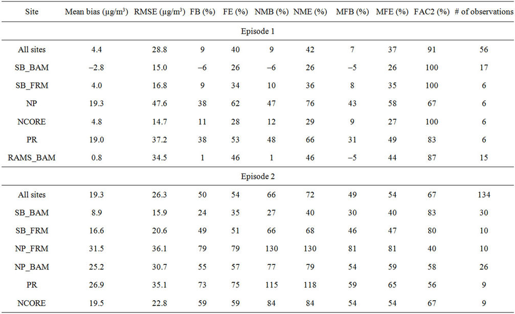
Table 3. Skill scores of CMAQ in simulating 24 h-average PM2.5-concentration as obtained at various sites where data were available during the two episodes.
within ±60% and MFE ≤ 75% are recommended as the criteria for a model’s performance to be considered as acceptable, and MFB within ±30% and MFE ≤ 50% are the goal that the best state-of-the-art models could reach [36]. For episode 1, 66% and 100% of the pairs of NMB-NME obtained at all stationary sites fell within the EPA [44] recommended performance goals and criteria (Table 3). In episode 2, only the pair of NMB-NME at the SB-site reached the performance goal, while the pairs of NMB-NME at other sites felt outside the performance criteria. Based on the criteria and skill-scores, we conclude that CMAQ’s performance was good for episode 1 and acceptable for episode 2.
For both episodes, CMAQ simulated the PM2.5-concentrations at the SB-site better than at other sites. Here its performance was better for episode 1 than 2 (Table 3, Figure 5). The slight temporal offset in simulated meteorology propagated into the simulated 24 h-average PM2.5-concentrations from December 27 to 31, 2009 (Figure 5). The overestimation of PM2.5 between January 7 and 9, 2011 was mainly caused by errors in emission allocations rather than by errors in simulated meteorology.
The evaluation of CMAQ-simulated PM2.5-concentrations with the PM2.5-concentrations measured by the sniffer during all drives of episode 1 yielded a mean bias, RMSE, FB, FE, NMB, NME, MFB, MFE and FAC2 of 3.0 µg/m3, 50.8 µg/m3, −4%, 94%, 8.5%, 93%, −4%, 94% and 39% respectively. The corresponding skill-scores in episode 2 were 11.5 µg/m3, 43.0 µg/m3, 10%, 105%, 42%, 118%, 10%, 105% and 28%. The skill-scores obtained in episode 1 (2) are better (slightly weaker) than those obtained in other studies for this region [28]. Comparison of the skill-scores obtained at the SB of episode 1 (2) with those reported at that site for an episode in January 2008 fall in the same range (are slightly weaker) [9]. The skill-scores determined for individual sniffer drives differed strongly from each other. CMAQ typically performed better on days with high
(>30 µg/m3 on average) than low PM2.5-concentrations detected by the sniffer. Highest correlation between simulated and sniffer-observed PM2.5-concentrations obtained for any drive was 0.824 (statistically significant), but typically varied ±0.200 (occasionally statistical significant). Some of the discrepancies are due to the fact that simulated PM2.5-concentrations represent volumeaverage concentrations for 1.3 km × 1.3 km × 8 m, while the “sniffer observations” represent the average along the route (a line) within that grid-cell at the same hour.
4.3. Evaluation of the Tool
For episode 1, the cross-evaluation of our interpolation tool yielded FB, FE, NMB, NME, MFE, MFB, FAC2 and R over all grid-cells with mobile measurements and all drives of 4%, 42%, 4%, 43%, 8%, 58%, 68%, and 0.728, respectively. The corresponding values for episode 2 were 4%, 40%, 5%, 41%, 2%, 45%, 77% and 0.707 (Figure 6).
The skill-scores differ among drives in episodes 1 and 2.
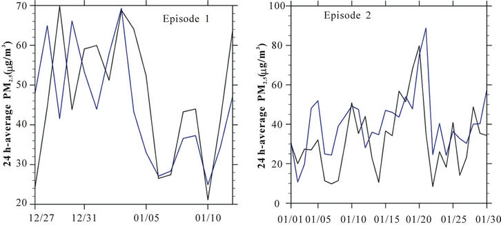
Figure 5. Temporal evolution of simulated (blue) and observed (black) 24 h-average PM2.5-concentrations as obtained at the SB-site for episodes 1 and 2, respectively.
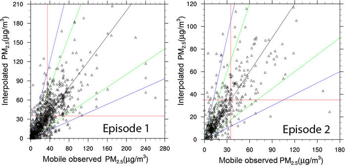
Figure 6. Scatter plots of interpolated and mobile observed PM2.5-concentrations at grid-cells on all routes of episodes 1 and 2. The black, green and blue lines indicate the 1:1-line and a factor of two and three agreement between pairs of simulated and observed values, respectively. The red lines indicate the PM2.5-NAAQS of 35 µg/m3.
The relatively strong (>0.7; statistically significant) correlations between the interpolated and observed concentrations for the various routes indicate that the interpolation algorithm captures the spatial distribution of observed PM2.5-concentrations along the routes well. Typically, skill-scores were better for days on which the snifffer measured high than low PM2.5-concentrations.
We also performed the cross-validation at grid-cells that the sniffer frequently travelled (≥20 times) during episodes 1 and 2. At these grid-cells, typical ranges of the performance skill-scores were −33% < FB < 29%, 10% < FE < 58%, −30% < NMB < 10%, 15% < NME < 50%, −43% < MFB < 33%, 20% < MFE < 72%, 54% < FAC2 < 96% and 0.400 < R < 0.920 (all correlations are statistically significant), respectively. These scores indicate that the tool even can capture the temporal evolution of the concentrations.
The evaluation of the interpolation tool by data from the SB-site provided overall FB, FE, NMB, NME, MFB, MFE, FAC2 and R of −67%, 78%, −50%, 59%, −69%, −80%, 39% and 0.341 (statistically significant), respecttively. The corresponding skill scores obtained at the NP- (RAMS-) site were 29% (39%), 70% (92%), 33% (48%), 82% (115%), 17% (−5%), 68% (85%), 50% (41%) and 0.215 (−0.120, both correlations statistically insignificant), respectively.
The relatively large discrepancy between the PM2.5- concentrations interpolated from the mobile measurements to the fixed sites may be partly explained by the large differences between the PM2.5-concentrations observed by the sniffer and at the fixed sites. More than 65% of the times when the measurements on the route were made in a grid-cell with a fixed site, the mobile and fixed site observations differed up to two orders of magnitude (Figure 7). This discrepancy can be explained by
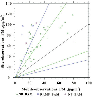
Figure 7. Like Figure 6, but for site-observations and mobile-observations at times when they were measured at same grid-cell in the route.
the fact that the mobile measurements are made along a line, while the site measurements are point measurements and at higher elevation than the sniffer measurements.
As aforementioned, the equations for the interpolation algorithm were developed using the CMAQ-data of episode 1. We used CMAQ-data for episode 2 as the “grand truth” for the evaluation of the tool’s accuracy to ensure independence of the data used for development and evaluation. Typically, the performance skill scores for the interpolation algorithm over all routes for grid-cells adjacent to the routes were R > 0.8, −10% < FB < 10%, FE < 30%, −20% < NMB < 20%, NME < 20%, −20% < MFB < 20%, MFE < 40%, FAC2 > 75%.
The comparison of interpolated and simulated “grand truth” PM2.5-concentrations revealed a sensitivity of the tool’s performance to the routes. The performance was weakest when the route only covered a few grid-cells (<10), or just one side of the nonattainment area, for instance, the community of North Pole, or the hills (Figure 8). The tool performed best (weakest) for routes that covered the center of nonattainment (the hills). However, since in the hills, PM2.5-concentrations are usually below the NAAQS, the relatively weaker performance here than elsewhere will not lead to false alarms, i.e. notifications of unhealthy conditions when there are actually none.
We examined the overall accuracy of the tool over 100 randomly chosen routes for episode 2. In doing so, we randomly picked a day of episode 2 and used the PM2.5-concentrations simulated by CMAQ for that day as “grand truth”. For that day we also randomly picked a route. We extracted the PM2.5-concentrations on this route as measurements from the “grand truth”. Then we applied the tool for this route and interpolated the extracted PM2.5-concentrations into the neighborhoods. We repeated this procedure 100 times. These 100 interpolated PM2.5-concentration datasets were then evaluated with the corresponding “grand truth” CMAQ-simulated PM2.5-concentrations. This evaluation led to R > 0.720, −20 < FB < 20, FE < 60%, −30% < NMB < 30%, NME < 50%, −30% < MFB < 30%, MFE < 60%, and FAC2 > 75% for most locations in the nonattainment area on average over all 100 samples (Figure 9).
The sensitivity study on the wind-direction dependent interpolation algorithm suggested that consideration of wind-direction does not improve the performance (therefore not shown). The same result was found for the algorithm with consideration of wind-speed. Comparison of the wind observations made at the meteorological tower with those made at Fairbanks International Airport, Eielson Air Force Base and Fort Wainwright suggested that the meteorological tower is not very representative for the wind pattern over the nonattainment area. This finding also agrees with other studies made for Fairbanks [45].
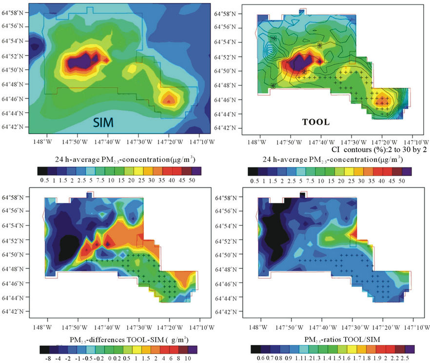
Figure 8. Example of interpolated (TOOL) vs. simulated, i.e. “grand truth”, (SIM) PM2.5-concentrations as obtained with the developed interpolation algorithm using the CMAQ-data pulled at grid-cells on the actual route performed on 01/06/2011 as “proxy” for sniffer observations in the nonattainment area (see text for details). The red polygon indicates the Fairbanks PM2.5-nonattainment area. The black crosses indicate the grid-cells on the route for this day.
The consideration of a temperature-classification in the interpolation algorithm improved the performance in interpolating PM2.5-concentration in the hills. However, it led to decreased performance in downtown Fairbanks and the community of North Pole that are the two hotspot areas for high PM2.5-concentrations [28]. As in the hills, PM2.5-concentrations are usually below the NAAQS, and the PM2.5 hot-spots are of greatest public concerns, the interpolation algorithm without consideration of meteorological quantities seems to be the most suitable for public air-quality advisory on polluted days.
5. Transferability
The CMAQ-database of the tool developed in this study based on simulations for Fairbanks for one episode in deep winter with calm wind and extremely low temperature conditions. Note that such conditions are typical candidates for exceedances of the NAAQS at the SB-site
[4] and hence suitable for an interpolation algorithm aiming at providing a spatially differentiated air-quality advisory on such days.
Meteorological conditions as well as the emissions of PM2.5 and its precursors differ with season and location. Therefore, to apply the tool for a different season, the database of air-quality model simulations has to be enlarged for that season. If the tool is to be transferred to another region, a database has to be created from airquality model simulations for the respective region and season of interest.
To demonstrate the transferability of the developed tool, we created a PM2.5-concentration database from simulations of the WRF with inline chemistry package (WRF/Chem; [7]) in its Alaska adapted version [21] for an episode in May/June 2008 for a domain of 110 × 110 grid-cells with a 7 km increment over Southeast Alaska (Figure 10). We used ten days of the episode (May 15 to May 24, 2008) to create a database for the tool. This database includes 240 data at each grid-cell in total 2,851,440 values. Another 15 days (May 25 to June 8,
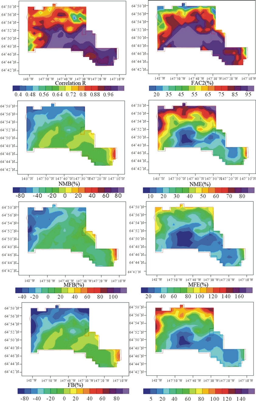
Figure 9. Overall performance of the interpolation algorithm as obtained on average over 100 arbitrarily chosen routes.
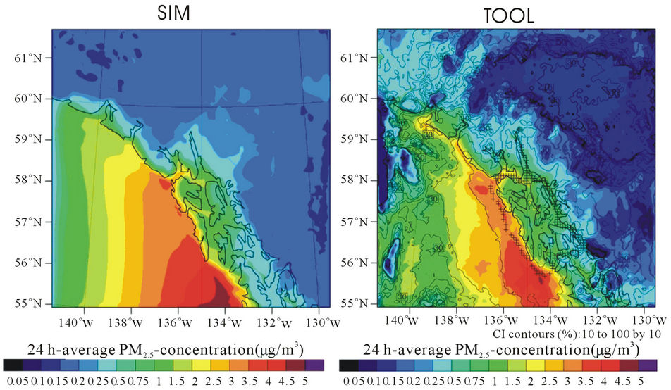
Figure 10. Example of interpolated (TOOL) vs. simulated, i.e. “grand truth”, (SIM) PM2.5-concentrations on May 28, 2008 as obtained with the developed interpolation algorithm using WRF/Chem-data as “proxy” for observation in Southeast Alaska (see text for details). The plus signs indicate the assumed route of an instrumented ship cruising on this day.
2008) were used as “grand truth” as there were no mobile measurements for this region. We assumed arbitrary routes of an instrumented ship that travels and measures PM2.5-concentrations around the islands in the domain during the 15 “grand truth” days (Figure 10). We extracted the PM2.5-concentrations along the assumed route from the “grand truth” data as “proxy” data of observations. Like in the evaluation of the interpolation tool, we used the database to build the interpolation equations, and interpolated the “observations”. Then the interpolated PM2.5-concentrations were evaluated with WRF/ Chem-simulated PM2.5-concentrations that we assumed as “grand truth” (Figure 10). This evaluation showed that the interpolation procedure captured the spatial distribution and magnitude of the “grand truth” PM2.5-concentrations well (Figure 10). Except at grid-cells on and near the route, the uncertainties were greater than 30% everywhere, especially at grid-cells where the PM2.5-concentration were low (<1 µg/m3). Over all seven assumed instrumented ship cruises during the 15 “grand truth” days, the tool generally performed well over the domain. The performance skill-scores fell in the following ranges: 0.34 < R < 1.0, −60% < FB < 60%, 5% < FE < 180%, −40% < NMB < 120%, 5% < NME < 180%, −80% < MFB < 140%, 5% < MFE < 160%, and 20% < FAC2 < 100% (Figure 11).
In some regions of the domain, the performance was relatively weak (Figure 11) due to the drastic changes in the meteorological conditions between the days used as database (May 15 to 24) and the days used as “grand truth” (May 25 to June 8). For instance, there was a change in wind-direction. From May 15 to 24 2008, land-sea-breeze circulations, mainly in west-east direction, dominated. On May 17 and 18, west wind dominated and advected aged polluted air from the ocean deep land inwards. From May 26 to 31, northern winds interfered with the land-sea-breeze circulations. Starting from June 1, the south and southeast winds interfered with and eventually shut down the land-sea-breezes. Because of this change, the spatial distribution of PM2.5-concentration in the database did not well represent the conditions of the “grand truth” days, for which the performance of the tool is weaker after the change occurred.
This transferability experiment illustrates the following: The tool can be easily transferred to other regions. Even with a large database, the ability of the tool is limited when the conditions at the time of the “measurements” differ strongly from the condition from which the interpolation equations were derived.
6. Conclusions
A tool to interpolate mobile PM2.5-measurements into unmonitored neighborhoods is presented. The tool uses simulations by the Alaska adapted CMAQ [9] or any other air-quality model as a database and the GPS-coor-
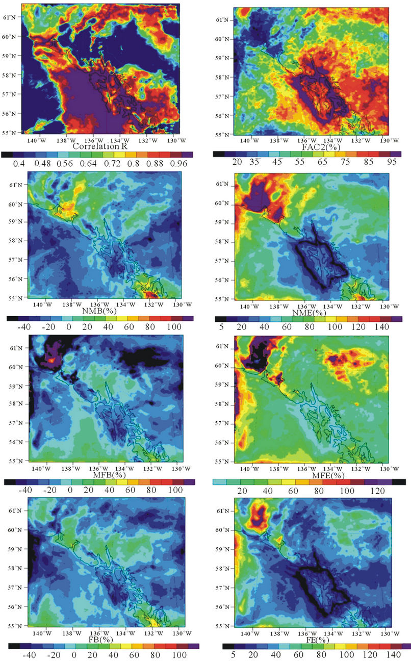
Figure 11. Overall performance of the interpolation performance as obtained over seven assumed instrumented ship cruises from May 25 to June 8, 2008 using WRF/Chem-data as “proxy” for observation in Southeast Alaska (see text for details).
dinates of the route to determine a set of interpolation equations for the neighborhood of interest, e.g. a nonattainment area. Once the interpolation equations are determined, the tool interpolates the mobile measurements into the unmonitored neighborhoods using the set of interpolation equations. The resulting concentration distributions can be used for spatially differentiated public air-quality advisory.
The tool allows any route within the area for which a database of simulated concentrations exits. The tool is transferable into other regions and seasons pre-assumed a database of air-quality simulations exists or is established for that region and/or season. A great advantage of this tool is that its database just needs to have values in the range of the mobile measured concentrations and to represent similar seasonal conditions in the region of interest. The tool does not require a simulation of the episode of the actual mobile measurements. Consequently, the spatial interpolation can be made within minutes after the end of a drive.
The results of cross-validations suggested that the interpolation algorithm performs best for grid-cells close to the route. The evaluation by using a CMAQ-simulation as “grand-truth” that has not been included in the database and hence for the determination of the interpolation equations showed that the interpolation algorithm captured the spatial distribution of the “grand-truth” PM2.5- concentrations well.
The evaluation efforts also showed that the performance of the tool is sensitive to the route. Performance is best for routes with large coverage of the region into which the mobile measurements are to be interpolated.
Sensitivity studies that included wind fields and temperature into the determination of the interpolation equations led to the conclusion that in a complex urban environment under calm wind conditions, a simpler algorithm that only considers PM2.5-concentrations is superior for capturing the conditions in hot-spot areas.
Our investigations showed that the tool does not need simulations of the actual day of the mobile measurements to interpolate measurements successfully into unmonitored neighborhoods. This fact is of great advantage for public air-quality advisory as it tremendously reduces the time between the end of the measurements and the time the advisory can be released.
The tool presented here provides the flexibility for all types of routes, i.e. it is not tied to a specific route. Based on the transferability tests to southeast Alaska, one has to conclude that this tool can easily be applied to other regions and seasons. To apply the tool for another season, the database of air-quality model data must be enlarged by results from simulations representative for the season in the region of interest. The tool developed and evaluated in this study was based on 2592 concentrations at each grid-cell in the CMAQ-database. A reduction of this database by 30% reduces the tool’s accuracy by 10%.
7. Acknowledgements
We thank G. Kramm, G.A. Grell, and the anonymous reviewers for fruitful discussions. We thank J. Conner, J. McCormick, and N. Swensgard from the Fairbanks North Star Borough Air Quality Division for access to their PM2.5-data and Sierra Research Inc. for providing the emission data. The Arctic Super Computer Center provided computational support. The study was supported partly under the AUTC Project No. 410003 by the Alaska Department of Transportation & Public Facilities and the National Park Service under contract H9910030024.
REFERENCES
- H. N. Q. Tran and N. Mölders, “Investigations on Meteorological Conditions for Elevated PM2.5 in Fairbanks, Alaska,” Atmospheric Research, Vol. 99, No. 1, 2011, pp. 39-49. doi:10.1016/j.atmosres.2010.08.028
- D. W. Wong, L. Yuan and S. A. Perlin, “Comparison of Spatial Interpolation Methods for the Estimation of Air Quality Data,” Journal of Exposure Analysis and Environmental Epidemiology, Vol. 14, No. 5, 2004, pp. 404- 415. doi:10.1038/sj.jea.7500338
- J. A. Mulholland, A. J. Butler, J. G. Wilkinson and A. G. Russell, “Temporal and Spatial Distributions of Ozone in Atlanta: Regulatory and Epidemiologic Implications,” Journal of Air & Waste Management Association, Vol. 48, No. 5, 1998, pp. 418-426. doi:10.1080/10473289.1998.10463695
- D. PaiMazumder and N. Mölders, “Theoretical Assessment of Uncertainty in Regional Averages Due to Network Density and Design,” Journal of Applied Meteorology and Climate, Vol. 48, No. 8, 2009, pp. 1643-1666.
- J. F. Clarke, E. S. Edgerton and B. E. Martin, “Dry Deposition Calculations for the Clean Air Status and Trends Network,” Atmospheric Environment, Vol. 31, No. 21, 1997, pp. 3667-3678. doi:10.1016/S1352-2310(97)00141-6
- M. Fuentes and A. E. Raftery, “Model Evaluation and Spatial Interpolation by Bayesian Combination of Observations with Outputs from Numerical Models,” Biometrics, Vol. 61, No. 1, 2005, pp. 36-45. doi:10.1111/j.0006-341X.2005.030821.x
- S. E. Peckham, J. D. Fast, R. Schmitz, G. A. Grell, W. I. Gustafson, S. A. McKeen, S. J. Ghan, R. Zaveri, R. C. Easter, J. Barnard, E. Chapman, M. Salzmann, C. Wiedinmyer and S. R. Freitas, “WRF/Chem Version 3.1 User’s Guide,” 2009. http://ruc.noaa.gov/wrf/WG11/Users_guide.pdf
- D. W. Byun and K. L. Schere, “Review of the Governing Equations, Computational Algorithms, and Other Components of the Models-3 Community Multiscale Air Quality (CMAQ) Modeling System,” Applied Mechanics Reviews, Vol. 59, No. 2, 2006, pp. 51-77. doi:10.1115/1.2128636
- N. Mölders and K. Leelasakultum, “CMAQ Modeling: Final Report Phase I,” 2011, p. 62.
- B. J. Gaudet and D. R. Stauffer, “Stable Boundary Layers Representation in Meteorological Models in Extremely Cold Wintertime Conditions,” Report to the US Environmental Protection Agency, 2010, p. 60.
- S.-Y. Hong and J.-O. J. Lim, “The WRF Single-Moment 6-Class Microphysics Scheme (WSM),” Journal Korean Meteorological Society, Vol. 42, No. 2, 2006, pp. 129- 151.
- G. A. Grell and D. Dévényi, “A Generalized Approach to Parameterizing Convection Combining Ensemble and Data Assimilation Techniques,” Geophysical Research Letters, Vol. 29, No. 14, 1693, 2002, p. 4.
- M.-D. Chou and M. J. Suarez, “An Efficient Thermal Infrared Radiation Parameterization for Use in General Circulation Models,” NASA—Technical Memorandum, Vol. 3, No. 3, 1994, p. 85.
- E. J. Mlawer, S. J. Taubman, P. D. Brown, M. J. Iacono and S. A. Clough, “Radiative Transfer for Inhomogeneous Atmospheres: Rrtm, a Validated Correlated-K Model for the Longwave,” Journal of Geophysical Research, Vol. 102, No. D14, 1997, pp. 16663-16682. doi:16610.11029/16697JD00237
- J. Barnard, J. Fast, G. Paredes-Miranda, W. Arnott and A. Laskin, “Technical Note: Evaluation of the WRF-Chem ‘Aerosol Chemical to Aerosol Optical Properties’ Module Using Data from the Milagro Campaign,” Atmospheric Chemistry and Physics, Vol. 10, No. 15, 2010, pp. 7325- 7340. doi:10.5194/acp-10-7325-2010
- Z. I. Janjić, “The Step-Mountain Eta Coordinate Model: Further Developments of the Convection, Viscous Sublayer and Turbulence Closure Schemes,” Monthly Weather Review, Vol. 122, No. 5, 1994, pp. 927-945. doi:10.1175/1520-0493(1994)122<0927:TSMECM>2.0.CO;2
- T. G. Smirnova, J. M. Brown, S. G. Benjamin and D. Kim, “Parameterization of Cold Season Processes in the Maps Land-Surface Scheme,” Journal of Geophysical Research, Vol. 105, No. D3, 2000, pp. 4077-4086. doi:4010.1029/1999JD901047
- N. Mölders and G. Kramm, “Influence of Wildfire Induced Land-Cover Changes on Clouds and Precipitation in Interior Alaska—A Case Study,” Atmospheric Research, Vol. 84, No. 2, 2007, pp. 142-168. doi:10.1016/j.atmosres.2006.06.004
- N. Mölders and G. Kramm, “A Case Study on Wintertime Inversions in Interior Alaska with WRF,” Atmospheric Research, Vol. 95, No. 2-3, 2010, pp. 314-332. doi:10.1016/j.atmosres.2009.06.002
- D. W. Byun, J. E. Pleim, R. T. Tang and A. Bourgeois, “Science Algorithms of the Epa Models-3 Community Multiscale Air Quality (CMAQ) Modeling System— Chapter 12: Meteorology-Chemistry Interface Processor (MCIP) for CMAQ Modeling System,” Technical Report to US Environmental Protection Agency, 1999, p. 91.
- G. Yarwood, S. Rao, M. Yocke and G. Z. Whitten, “Updates to the Carbon Bond Chemical Machanism: CB05,” Final Report to the US Environmental Protection Agency, 2005. http://www.camx.com
- F. S. Binkowski and S. J. Roselle, “Models-3 Community Multiscale Air Quality (CMAQ) Model Aerosol Component, 1, Model Description,” Journal of Geophysical Research, Vol. 108, No. D6, 2003, p. 18. doi:10.1029/2001JD001409
- J. S. Chang, R. A. Brost, I. S. A. Isaksen, S. Madronich, P. Middleton, W. R. Stockwell and C. J. Walcek, “A ThreeDimensional Euledan Acid Deposition Model: Physical Concepts and Formulation,” Journal Geophysical Research, Vol. 92, No. D12, 1987, pp. 14681-14700. doi:10.1029/JD092iD12p14681
- B. Schell, I. J. Ackermann, H. Hass, F. S. Binkowski and A. Ebel, “Modeling the Formation of Secondary Organic Aerosol within a Comprehensive Air Quality Model System,” Journal of Geophysical Research, Vol. 106, No. D22, 2001, pp. 28275-28293. doi:28210.21029/22001JD000384
- R. J. Yamartino, “Nonnegative, Conserved Scalar Transport Using Grid-Cell-Centered, Spectrally Constrained Blackman Cubics for Applications on a Variable-Thickness Mesh,” Monthly Weather Review, Vol. 121, No. 3, 1993, pp. 753-763. doi:10.1175/1520-0493
- J. E. Pleim and J. S. Chang, “A Non-Local Closure Model for Vertical Mixing in the Convective Boundary Layer,” Atmospheric Environment, Vol. 26A, No. 6, 1992, pp. 965- 981.
- N. Mölders, H. N. Q. Tran, P. Quinn, K. Sassen, G. E. Shaw and G. Kramm, “Assessment of WRF/Chem to Simulate Sub-Arctic Boundary Layer Characteristics During Low Solar Irradiation Using Radiosonde, Sodar, and Surface Data,” Atmospheric Pollution Research, Vol. 2, 2011, pp. 283-299. doi:10.5094/APR.2011.035
- N. Mölders, H. N. Q. Tran, C. F. Cahill, K. Leelasakultum and T. T. Tran, “Assessment of WRF/Chem PM2.5- Forecasts Using Mobile and Fixed Location Data from the Fairbanks, Alaska Winter 2008/09 Field Campaign,” Atmospheric Pollution Research, Vol. 3, 2012, pp. 180- 191. doi:10.5094/APR.2012.018
- C. J. Coast Jr., “High-Performance Algorithms in the Sparse Matrix Operator Kernel Emissions (Smoke) Modeling System,” Ninth AMS Joint Conference on Applications of Air Pollution Meteorology with A&WMA, 1996, pp. 584-588.
- M. R. Houyoux, J. M. Vukovich, C. J. Coats, N. J. M. Wheeler and P. S. Kasibhatla, “Emission Inventory Development and Processing for the Seasonal Model for Regional Air Quality (Smraq) Project,” Journal of Geophysical Research, Vol. 105, No. D7, 2000, pp. 9079- 9090. doi:10.1029/1999JD900975
- N. Mölders, H. N. Q. Tran and K. Leelasakultum, “Investigation of Means for PM2.5 Mitigation through Atmospheric Modeling—Final Report,” 2011, p. 75.
- C. F. Cahill, “Asian Aerosol Transport to Alaska during ACE-Asia,” Journal of Geophysical Research, Vol. 108, No. 8664, 2003, p. 8.
- T. T. Tran, G. Newby and N. Mölders, “Impacts of Emission Changes on Sulfate Aerosols in Alaska,” Atmospheric Environment, Vol. 45, No. 18, 2011, pp. 3078- 3090. doi:10.1016/j.atmosenv.2011.03.013
- H. von Storch and F. W. Zwiers, “Statistical Analysis in Climate Research,” Cambridge University Press, Cambridge, 1999.
- J. C. Chang and S. R. Hanna, “Air Quality Model Performance Evaluation,” Meteorology and Atmospheric Physics, Vol. 87, No. 1-3, 2004, pp. 167-196. doi:10.1007/s00703-003-0070-7
- J. W. Boylan and A. G. Russell, “PM and Light Extinction Model Performance Metrics, Goals, and Criteria for Three-Dimensional Air Quality Models,” Atmospheric Environment, Vol. 40, No. 26, 2006, pp. 4946-4959. doi:10.1016/j.atmosenv.2005.09.087
- J. Devore, “Probability and Statistics for Engineering and the Sciences,” 6th Edition, Brooks/Cole, Belmont, 2004.
- S. Weisberg, “Applied Linear Regression,” 3rd Edition, Wiley, New York, 2005. doi:10.1002/0471704091
- Y. Zhang, M. K. Dubey, S. C. Olsen, J. Zheng and R. Zhang, “Comparisons of WRF/Chem Simulations in Mexico City with Ground-Based Rama Measurements during the 2006-Milagro,” Atmospheric Chemistry and Physics, Vol. 9, No. 11, 2009, pp. 3777-3798. doi:10.5194/acp-9-3777-2009
- Z. Zhao, S.-H. Chen, M. J. Kleeman, M. Tyree and D. Cayan, “The Impact of Climate Change on Air QualityRelated Meteorological Conditions in California. Part I: Present Time Simulation Analysis,” Journal Climate, Vol. 24, No. 13, 2011, pp. 3344-3361. doi:10.1175/2011JCLI3849.1
- N. Mölders, “Suitability of the Weather Research and Forecasting (WRF) Model to Predict the June 2005 Fire Weather for Interior Alaska,” Weather and Forecasting, Vol. 23, No. 5, 2008, pp. 953-973. doi:10.1175/2008WAF2007062.1
- N. Mölders, “Comparison of Canadian Forest Fire Danger Rating System and National Fire Danger Rating System Fire Indices Derived from Weather Research and Forecasting (WRF) Model Data for the June 2005 Interior Alaska Wildfires,” Atmospheric Research, Vol. 95, No. 2-3, 2010, pp. 290-306. doi:10.1016/j.atmosres.2009.03.010
- M. B. Yarker, D. PaiMazumder, C. F. Cahill, J. Dehn, A. Prakash and N. Mölders, “Theoretical Investigations on Potential Impacts of High-Latitude Volcanic Emissions of Heat, Aerosols and Water Vapor and Their Interactions on Clouds and Precipitation,” The Open Atmospheric Science Journal, Vol. 4, No. 1, 2010, pp. 24-44. doi:10.2174/1874282301004010024
- U. S. EPA, “Guidance on the Use of Models and Other Analyses for Demonstrating Attainment of Air Quality Goals for Ozone, PM2.5, and Regional Haze,” Research Triangle Park, North Carolina, 2007, p. 262.
- H. N. Q. Tran and N. Mölders, “Wood-Burning Device Changeout: Modeling the Impact on PM2.5-Concentrations in a Remote Subarctic Urban Nonattainment Area,” Advances in Meteorology, 2012, 12 Pages, Article ID: 853405. doi:10.1155/2012/853405
NOTES
*Corresponding author.