Smart Grid and Renewable Energy
Vol.2 No.4(2011), Article ID:8415,8 pages DOI:10.4236/sgre.2011.24041
Online One-End Fault Location Algorithm for Parallel Transmission Lines
![]()
Department of Electrical and Computer Engineering, University of Kentucky, Lexington, USA.
Email: yliao@engr.uky.edu
Received September 7th, 2011; revised October 10th, 2011; accepted October 18th, 2011.
Keywords: Distance Protection, Fault Location, Parallel Transmission Line
ABSTRACT
Fault location and distance protection are essential smart grid technologies ensuring reliability of the power system. This paper describes an accurate algorithm for locating faults on double-circuit transmission lines. The proposed approach is capable of identifying the faulted circuit of a parallel transmission line by checking the estimated fault location and fault resistance. Voltage and current measurements from only one of the terminals of the faulty line are used. No pre-fault data are required for the estimation. The lumped parameter line model considering shunt capacitance is utilized for the derivation of the algorithm. It’s assumed that line parameters are known and transmission lines are fully transposed. The method is applicable to all types of faults. It’s evinced by evaluation studies that the proposed algorithm can correctly determine the faulted circuit in most cases. For exceptional cases, the current waveforms during the fault can be used to help identify the faulted circuit. The proposed algorithm generates quite accurate fault location estimates, and may be suitable for distance relaying.
1. Introduction
To provide more reliable operations and higher power transfer capability, double circuit transmission lines are becoming more widely utilized in the power transmission systems. Since quick power system restoration and less outage time are important to the power grid, especially for the emerging smart grid, researchers developed various fault location algorithms for quick and accurate fault location on power transmission lines.
Most of the fault location approaches are based on voltage and current measurements acquired from one end or several ends of the lines. In papers [1-4], data from only one terminal of the faulted line are used for finding fault position on double-circuit lines. For double-circuit transmission lines, the mutual coupling between the adjacent lines can affect the fault location estimation considerably [5]. In order to solve this problem, authors of [1] made use of modal transformation technique to convert the coupled equations of transmission line into decoupled ones. As a result, the effects of mutual coupling as well as pre-fault currents and charging currents have been eliminated. A fault location algorithm, independent of source impedances, fault resistance and remote infeed is described in [2]. By using phase currents from both the sound and faulted circuits together with the phase voltages as the input signals, [4] provide fault location methods for iteratively compensating the effects of line shunt capacitances for enhanced accuracy.
Measurement data at both ends of the faulty line are fed to two-terminal methods for locating faults in [6,7]. A method described in [6] decomposes the parallel transmission line network into a differential component network and a common component network. Although very short data window is needed and any segment of the data after fault can be utilized as the input for the method, this algorithm is not applicable to all kinds of parallel transmission line systems. Reference [7] presents a fault location method based on distributed line model. However, phasor measurements units (PMU) for synchronized data and continuous monitoring of the line under normal operation are required.
Multi-terminal methods implemented with signals available from several buses are discussed in [8,9]. An approach proposed in [8] employs the magnitude of the differential currents at each terminal to locate the fault for multi-terminal two parallel transmission lines. Since fault location algorithms usually varies according to different fault types, Funabashi and et al. developed their method, in which for all types of faults, the equations used for pinpointing the fault location are the same [9].
Although two-terminal and multi-terminal methods usually produce more accurate results, one-terminal approaches still have advantages such as simplicity and no need for communication with remote end.
In recent years, some special methods for finding fault positions on parallel transmission lines are presented in [10,11]. As we know, most of the fault location algorithms for double circuit lines require measurements from at least one of the local terminals. One of the advantages of [10] is that only voltage measurements from one or two buses, which can be far from the faulted section, are needed. Due to this reason, the new approach can be taken as a method in case there is no data-recording device near the faulted line. Authors of [11] apply Artificial Neural Networks (ANNs) to fault analysis for fault detection, fault classification and fault location. For different aims of fault analysis, the particular Neural-network structure is selected with the help of a software tool named SARENEUR.
Generally speaking, the existing fault location methods are suitable for off-line analysis. This paper aims to present a method for online applications, which is capable of identifying the faulted circuit and locating the faults as well. In other words, the proposed method does not need to know which circuit of the parallel line is faulted. In this paper, in order to enhance the accuracy of the estimates, shunt capacitances of long lines are considered in the power system model utilized in [2]. It is assumed that the network data, including source impedances and transmission line parameters, are known. It is also assumed that power lines are fully transposed, and the positiveand negative-sequence line impedances are equal. Compared to [4], the proposed method in this paper solves one equation to directly obtain the fault location without the need to iteratively compensate the line shunt capacitances. Therefore, the proposed method may be suitable for online distance protection.
Section 2 presents the proposed fault location approaches with boundary condition for each type of fault. An online protection method for parallel transmission lines is discussed in detail as well. Simulation studies based on Electro-Magnetic Transients Program (EMTP) under diverse fault conditions are reported in Section 3 [12], followed by the conclusion.
2. Fault Location Algorithm for Parallel Transmission Lines
The system diagram adopted for deriving the new fault location algorithm is shown in Figure 1. Although the distributed parameter line model is more accurate for modeling lines than the nominal-PI model, the distributed
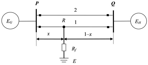
Figure 1. Circuit diagram used for developing the new algorithm.
parameter model is more computationally demanding. For the interests of computational efficiency, the nominal-PI model is utilized. Only voltage and current measurements at terminal P are used for estimating the fault location.
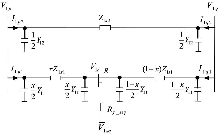
Positive, negative and zero sequence circuits of the system are depicted in Figure 2(a), Figure 2(b) and Figure 2(c), respectively. Suppose a fault with a fault resistance of  occurs on circuit 1 at location R. The following notations are defined for deriving the algorithm:
 zero, positive and negative sequence voltages at terminal P, respectively;
 zero, positive and negative sequence voltages at terminal Q, respectively;
 zero sequence voltages at bus R and F, respectively;
 positive and negative sequence voltages at bus R, respectively;
 zero, positive and negative sequence currents through circuit 1 at terminal P, respectively;
 zero, positive and negative sequence currents through circuit 2 at terminal P, respectively;
 zero, positive and negative sequence currents through circuit 1 at terminal Q, respectively;
 zero, positive and negative sequence currents through circuit 2 at terminal Q, respectively;
 zero, positive and negative sequence voltages at fault location E, respectively;
 total zero, positive and negative sequence series impedances of circuit 1 respectively and
 ;
;
 total zero, positive and negative sequence series impedances of circuit 2 respectively and
 ;
;
 total zero, positive and negative sequence shunt admittances of circuit 1 respectively and
 ;
;
 total zero, positive and negative sequence shunt admittances of circuit 2 respectively and
 ;
;
 total zero sequence mutual impedance between circuit 1 and circuit 2;
 total zero sequence mutual admittance between circuit 1 and circuit 2;
![]() fault distance from terminal P in per unit;
fault distance from terminal P in per unit;
 fault resistance in ohms;
 (a)
(a) (b)
(b)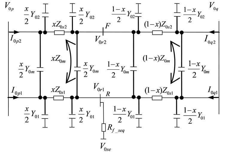 (c)
(c)
Figure 2. (a) Positive sequence circuit of the system. (b) Negative sequence circuit of the system. (c) Zero sequence circuit of the system.
 fault resistance shown in sequence circuits in ohms.
2.1. Sequence Equations
Known phase voltages and currents at terminal P, we can obtain the symmetrical components from phase components by employing the symmetrical component theory [13].
From the positive sequence network shown in Figure 2(a), the following equations are obtained based on the measurements at terminal P:
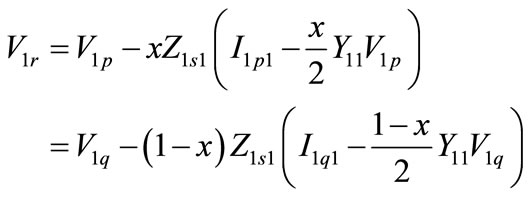 (1)
(1)
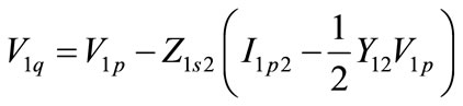 (2)
(2)
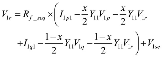 (3)
(3)
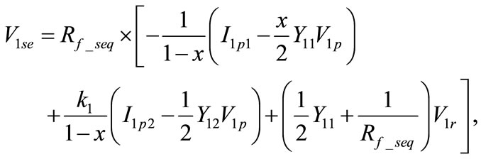
Eliminating  and
and  from Equations (1), (2) and (3), it yields
 (4)
(4)
where
 (5)
(5)
Similarly, for negative sequence network, the following equation is derived:
 (6)
(6)
For zero sequence circuit, the following four equations hold according to Figure 2(c):
 (7)
(7)
 (8)
(8)
 (9)
(9)
 (10)
(10)
Eliminating ,
,  and
and  from Equations (7), (8), (9) and (10), it follows
 (11)
(11)
where
 (12)
(12)
2.2. Boundary Conditions
In this section, boundary conditions for single line to ground (LG), line to line (LL), line to line to ground (LLG) and balanced three-phase (LLL) faults are described respectively with details. Newton-Raphson method is applied to estimate the fault location after the final equations are acquired.
2.2.1. Single Line to Ground Faults
Phase A to ground (AG) faults are taken as an instance for deriving the new algorithm. For AG faults, the boundary condition is given as
 (13)
(13)
Substituting Equations (4), (6), (11) into (13) leads to
 (14)
(14)
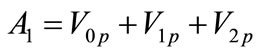
where  are constants defined in Appendix I.
Rearranging Equation (14), it becomes
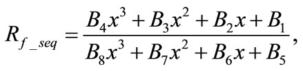 (15)
(15)
where  are constants defined in Appendix I.
Since  is the sequence fault resistance in ohms, it is a real number, or equivalently
 (16)
(16)
where the bar over a variable represents the its complex conjugate.
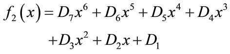
Substituting (15) into (16) results in
 (17)
(17)
 (18)
(18)
where  are constants defined in Appendix I.
By applying the Newton-Raphson method to function  as follows, fault location
 ![]() can be estimated accurately.
can be estimated accurately.
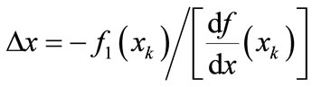 (19)
(19)
 (20)
(20)
where
 is the estimate of
 ![]() at the
at the  iteration;
 is the difference between two successive estimations;
 is the iteration number starting from 1.
An initial value of  for fault location can be adopted for the iterative approach. The iteration can be terminated when the desired tolerance for
 ![]() is reached. After
is reached. After ![]() is obtained, Equation (15) can be utilized to compute the value for
is obtained, Equation (15) can be utilized to compute the value for . Due to the calculated
  from Equation (15) may have negligible imaginary part, the real part of
  is taken as the final estimate for sequence fault resistance.
It’s worth noting that  is the fault resistance demonstrated in the sequence circuits while
  is the actual fault resistance for each type of fault. Under AG fault,
  is the resistance between phase A and the ground. In this case,
 .
.
The following procedure is utilized to determine which circuit of the parallel lines is faulted. First of all, we assume the fault occurs on circuit 1. Then, the proposed algorithm is employed to calculate the estimated ![]() and
and . If
. If ![]() is out of range from 0 to 1 or
is out of range from 0 to 1 or  is less than 0, it means the assumption is incorrect. Then, we run the algorithm again by assuming circuit 2 is the faulty circuit. Study results show that for various fault locations and resistances, this approach can successfully distinguish the sound and faulty circuits.
2.2.2. Line to Line Faults
Take phase B to phase C (BC) faults as an example. Phase B is connected to phase C though a fault resistance of . The boundary condition for BC faults is described as
 (21)
(21)
Substituting (4) and (6) into (21), similar function as (17) can be acquired:
 (22)
(22)
 (23)
(23)
where  are constants, which will not be provided with details in this paper.
By employing the Newton-Raphson approach to function , fault location
 ![]() can be well estimated and therefore
can be well estimated and therefore  can be obtained as well. For BC faults,
 .
.
2.2.3. Line to Line to Ground Faults
For line to line to ground faults, a phase B to phase C to ground (BCG) fault is discussed in details. In this case, both phase B and phase C are grounded through a resistance . For BCG faults, boundary condition is written as
 (24)
(24)
Since the boundary condition for BCG faults and BC faults are the same, we have identical equations for calculating fault location ![]() and sequence fault resistance
and sequence fault resistance .
.  under BCG faults.
2.2.4. Balanced Three-Phase Faults
For LLL faults, boundary condition is given as
 (25)
(25)
Because the boundary condition for LLL faults satisfies the boundary condition for BC faults, the same equations developed under BC faults can be used for LLL faults to estimate fault location ![]() and sequence fault resistance
and sequence fault resistance .
.  is equal to
  during balanced three-phase faults.
One distinctive feature of the developed algorithm is its capability to identify which circuit of the parallel line is faulted utilizing the following procedure. We will first assume that the fault falls on circuit 1 and applies the developed method. If the obtained fault location estimate is within zero and one and fault resistance estimate is larger than zero, it indicates that the assumption is correct. Otherwise, we will apply the developed method assuming that the fault occurs on circuit 2 to obtain a new pair of estimates. The evaluation studies presented in Section 3 illustrate this process.
3. Evaluation Studies
In this section, the EMTP package has been adopted to simulate a double-circuit line system under diverse fault conditions based on the distributed parameter line model [12]. A 50 Hz power system shown in Figure 3 is modeled for the study. The simulated power system consists of two generators at the two ends and a 200-mile parallel transmission line. One of the circuits is suffering from the fault. Generator information and line parameters are presented in Tables 1, 2 and 3. In this study, base values of 500 kV and 100 MVA are chosen for the per unit system. In the studies, all the simulated faults are placed on circuit 1.
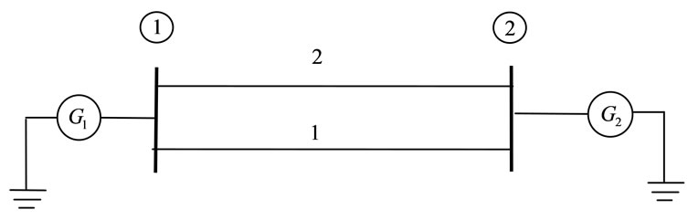
Figure 3. Schematic diagram of studied power system.
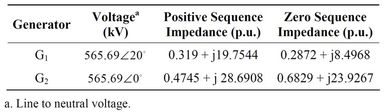
Table 1. Source impedance.
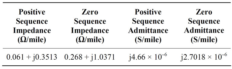
Table 2. Transmission line parameters for both circuits.
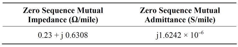
Table 3. Mutual coupling between circuit 1 and circuit 2.
Transient waveforms generated from EMTP are processed to obtain the voltage and current phasors. Fault location estimates are acquired by implementing the new algorithms in Matlab. Table 4 presents the results under various fault conditions when assuming faults occurring on circuit 1. In the table, ![]() is defined as the distance in per unit from the fault point on the faulty circuit to bus 1. The first three columns of Table 4 list the actual fault type, fault resistance and fault location, respectively. Fault location estimates are given in the fourth column in per unit. Evaluation studies indicate that all of the simulated faults are on circuit 1 and quite accurate estimates for fault location are generated by the algorithms.
is defined as the distance in per unit from the fault point on the faulty circuit to bus 1. The first three columns of Table 4 list the actual fault type, fault resistance and fault location, respectively. Fault location estimates are given in the fourth column in per unit. Evaluation studies indicate that all of the simulated faults are on circuit 1 and quite accurate estimates for fault location are generated by the algorithms.
As indicated in Section 2, the developed algorithm is capable of identifying which circuit of the parallel line is faulted. For instances, let us assume that the fault occurs on circuit 2, the fault location estimates are obtained as shown in Table 5. “N/A” indicates that an estimate of fault location within zero and one cannot be found. It is evinced that either the fault location estimate is out of the range from zero to one or the fault resistance estimate is less than zero and thus indicates that the fault does not occur on circuit 2, but occurs on circuit 1.
Sometimes, the algorithm can produce a valid solution if the fault is assumed to be on the actually healthy circuit. For example, for an AG fault occurring on circuit 1 at  with
with  ohm, if we assume the fault is on circuit 2, the proposed algorithm yields the estimate pair
  and
and  ohm, which is a valid solution. Under such circumstances, we cannot tell which circuit is the faulty one. More research is needed to find out under which fault conditions this phenomenon will occur. Under such circumstances, the current waveforms are utilized to identify the faulty circuit because the faulty circuit has larger currents than the healthy circuit due to the fault.
The method proposed in this paper generally yields higher accuracy than the method described in [2] for LL, LLG and LLL faults. For LG faults, the new method is more accurate if the fault resistance is larger than 100 ohms, but is not as accurate as the one in [2] for fault cases with smaller resistances. So for LG faults with small estimated fault resistances, the method in [2] can be applied.
4. Conclusions
A novel fault location algorithm considering shunt ca
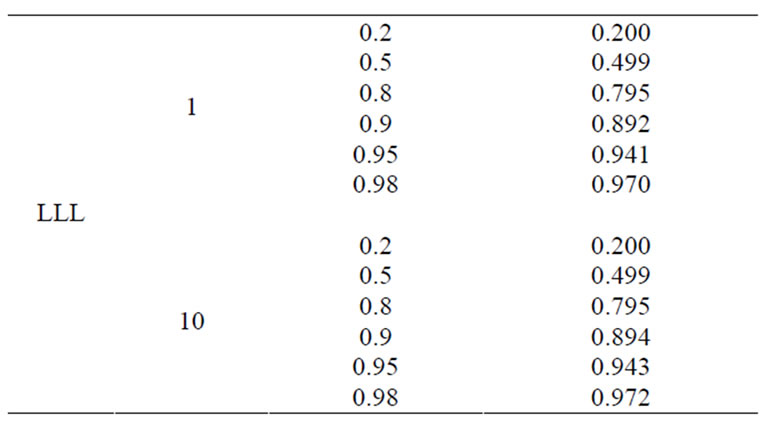
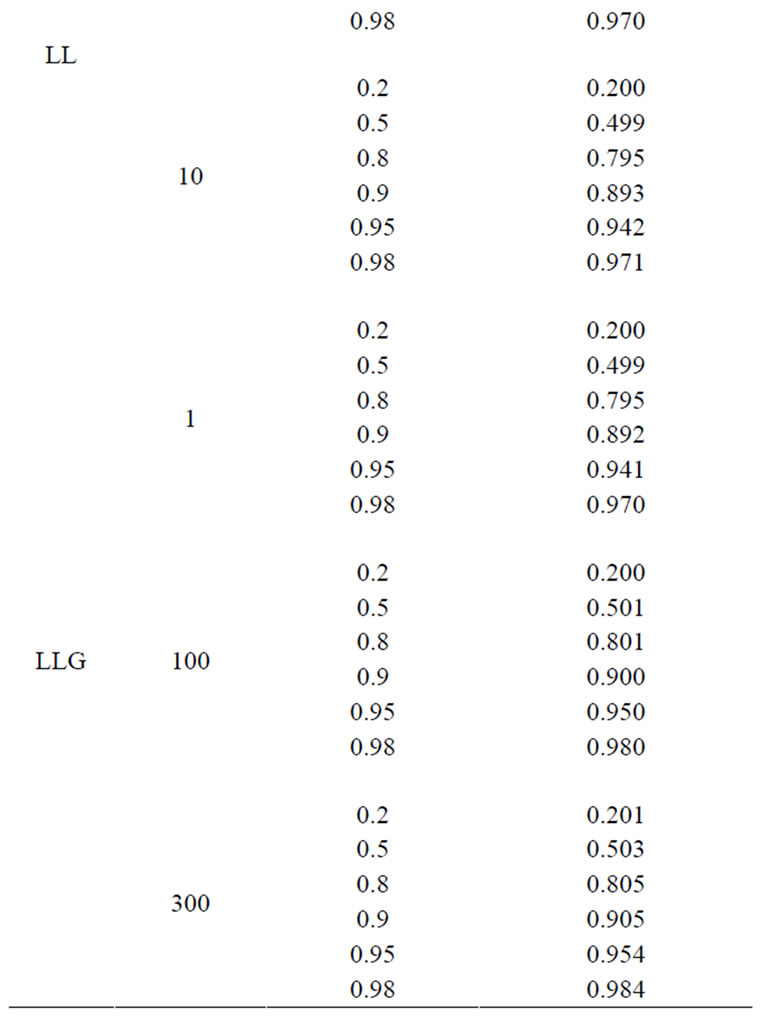

Table 4. Fault location results assuming faults occurring on circuit 1.
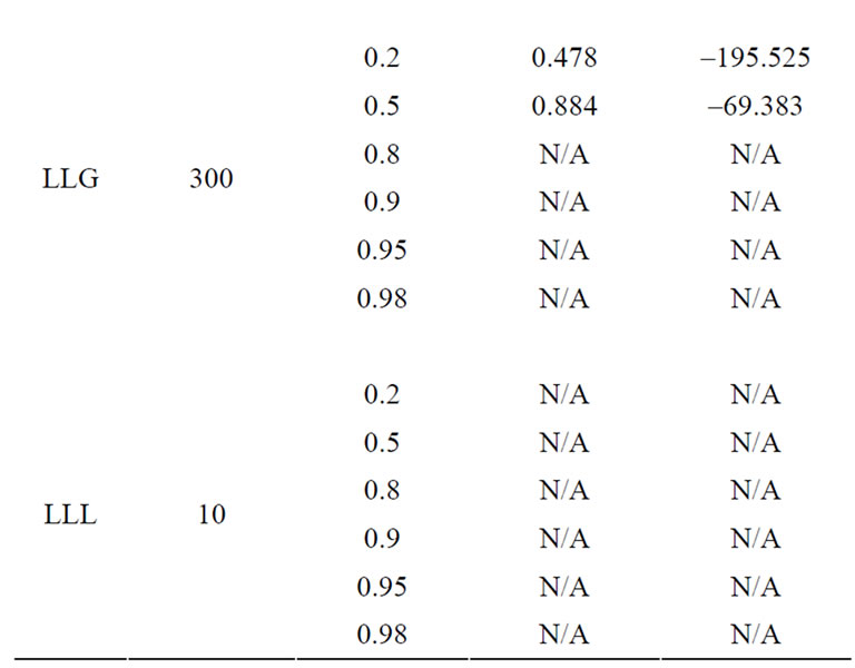
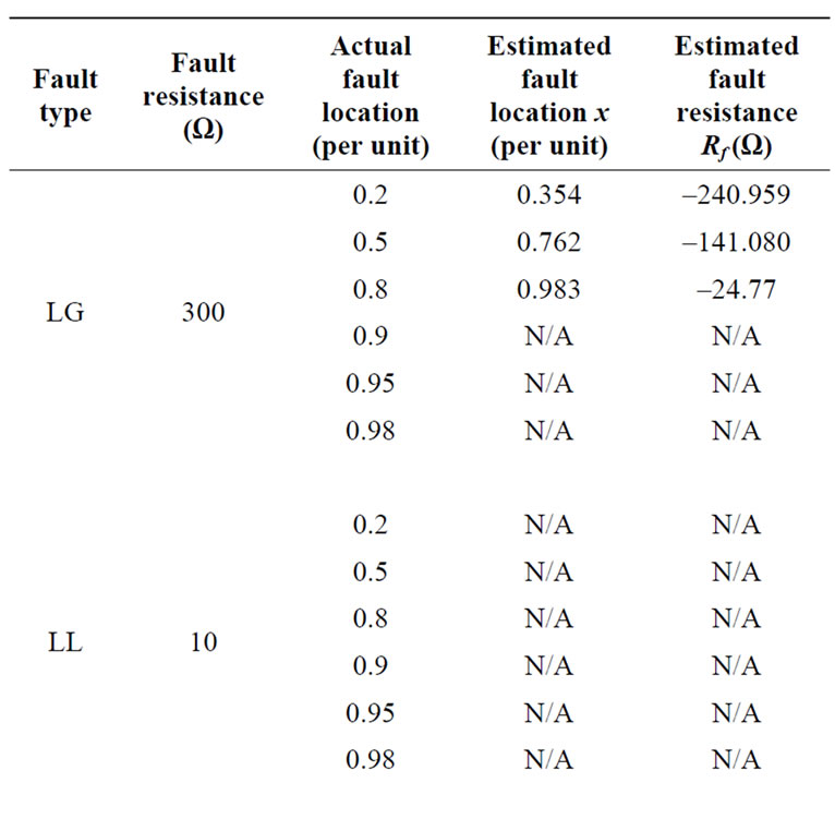
Table 5. Fault location results assuming faults occurring on circuit 2.
pacitance has been discussed in this paper. Only voltage and current measurements at one of the terminals are needed. No pre-fault data is required in the approach. Lumped parameter line model is used instead of the distributed line model for the interests of computational efficiency. The proposed algorithm may be utilized for online protection. By examining the estimated fault location and fault resistance obtained under a certain assumption, the new method can distinguish the sound and faulted circuits in most cases. Besides, the new approach, which is applicable to both symmetrical and unsymmetrical faults, is independent of source impendence and fault resistance. Simulation studies have demonstrated that the algorithm produces quite accurate estimates for all kinds of faults.
REFERENCES
- T. Kawady and J. Stenzel, “A Practical Fault Location Approach for Double Circuit Transmission Lines Using Single End Data,” IEEE Transactions on Power Delivery, Vol. 18, No. 4, 2003, pp. 1166-1173. doi:10.1109/TPWRD.2003.817503
- Y. Liao and S. Elangovan, “Digital Distance Relaying Algorithm for First-Zone Protection for Parallel Transmission Lines,” IEE Proceedings-Part C: Generation, Transmission and Distribution, Vol. 145, No. 5, 1998, pp. 531-536.
- Y. Ahn, M. Choi, S. Kang and S. Lee, “An Accurate Fault Location Algorithm for Double-Circuit Transmission Systems,” IEEE Power Engineering Society Summer Meeting, Seattle, 16-20 July 2000, pp. 1344-1349.
- J. Izykowski, E. Rosolowski and M. M. Saha, “Locating Faults in Parallel Transmission Lines under Availability of Complete Measurements at One End,” IEE Proceedings-Generation, Transmission and Distribution, Vol. 151, No. 2, 2004, pp. 268-273. doi:10.1049/ip-gtd:20040163
- Power System Relaying Committee, “Guide for Determining Fault Location on AC Transmission and Distribution Lines,” IEEE C37.114, 2005, pp. 1-36.
- G. Song, J. Suonan, Q. Xu, P. Chen and Y. Ge, “Parallel Transmission Lines Fault Location Algorithm Based on Differential Component Net,” IEEE Transactions on Power Delivery, Vol. 20, No. 4, 2005, pp. 2396-2406. doi:10.1109/TPWRD.2005.852364
- C. S. Chen, C. W. Liu and J. A. Jiang, “A New Adaptive PMU Based Protection Scheme for Transposed/Untransposed Parallel Transmission Lines,” IEEE Transactions on Power Delivery, Vol. 17, No. 2, 2002, pp. 395-404. doi:10.1109/61.997906
- T. Nagasawa, M. Abe, N. Otsuzuki, T. Emura, Y. Jikihara and M. Takeuchi, “Development of a New Fault Location Algorithm for Multi-Terminal Two Parallel Transmission Lines,” IEEE Transactions on Power Delivery, Vol. 7, No. 3, 1992, pp. 1516-1532. doi:10.1109/61.141872
- T. Funabashi, H. Otoguro, Y. Mizuma, L. Dube and A. Ametani, “Digital Fault Location for Parallel DoubleCircuit Multi-Terminal Transmission Lines,” IEEE Transactions on Power Delivery, Vol. 15, No. 2, 2000, pp. 531- 537. doi:10.1109/61.852980
- N. Kang and Y. Liao, “Fault Location for Double-Circuit Lines Utilizing Sparse Voltage Measurements,” Power & Energy Society General Meeting, Calgary, 26-30 July 2009, pp. 1-7.
- J. Gracia, A. J. Mazon and I. Zamora, “Best ANN Structures for Fault Location in Singleand Double-Circuit Transmission Lines,” IEEE Transactions on Power Delivery, Vol. 20, No. 4, 2005, pp. 2389-2395. doi:10.1109/TPWRD.2005.855482
- Leuven EMTP Centre, “Alternative Transient Program,” User Manual and Rule Book, Leuven, 1987.
- J. Grainger and W. Stevenson, “Power System Analysis,” McGraw-Hill Inc., New York, 1994.
Appendix I
 (A.1)
(A.1)
 (A.2)
(A.2)
 (A.3)
(A.3)
 (A.4)
(A.4)
 (A.5)
(A.5)
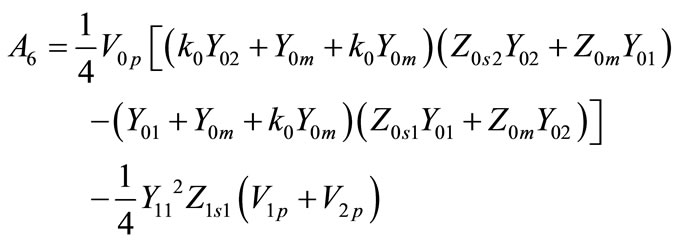 (A.6)
(A.6)
 (A.7)
(A.7)
 (A.8)
(A.8)
 (A.9)
(A.9)
 (A.10)
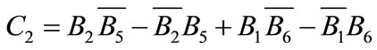
 (A.11)
 (A.12)
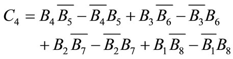
 (A.13)
 (A.14)
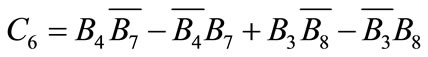
 (A.15)
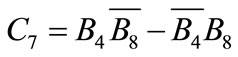
 (A.16)
 (A.17)
 (A.18)
 (A.19)
 (A.20)
 (A.21)