Smart Grid and Renewable Energy
Vol.2 No.3(2011), Article ID:6649,10 pages DOI:10.4236/sgre.2011.23027
Embedding PV and WF Models into Steady State Studies by an Optimization Strategy
![]()
Centro de Investigación y de Estudios Avanzados del I.P.N., Unidad Guadalajara, Zapopan, Mexico.
Email: jramirez@gdl.cinvestav.mx
Received March 16, 2011; revised April 13, 2011; accepted April 20, 2011.
Keywords: Distributed Generation (DG), Optimization, Photovoltaic Energy, Renewable Energy, Smart Grid, Wind Farm
ABSTRACT
Modeling of photovoltaic (PV) and wind farms (WF) stations to take into account these renewable energies into the power flow formulation are summarized. A strategy based on multi objective optimization in order to allocate PV and WF power into electrical power system is proposed. It is assumed that there are a reduced number of choices to allocate the stations. The algorithm is applied to the 39-bus test power system. The results show that the proposed algorithm is capable of optimal placement of renewable units.
1. Introduction
There is a tendency to transform the current electric power system (EPS) into a Smart Electrical Energy Network (SEEN). Future SEENs will be strong, more flexible, reliable, self-healing, fully controllable, assets efficient and will be a platform to make possible the coexistence of smart-self-controlling grids with great numbers of distributed generation systems (DGs) and large-scale centralized power plants. The need for modifications, demands to remove the barriers to the large-scale exploitation and integration of DGs and other players, will necessitate research and the development of innovative technologies from generation, transmission and distribution to communication tools, with far more sensors than at present. Thus, it is envisaged that flexible ac transmission systems (FACTS), energy storage systems (ESS), DGs, smart end-user appliances together with communications will be at the heart of the future SEENs [1].
We are mostly dependent on nonrenewable fossil fuels that have been and will continue to be a major cause of pollution and climate change. Because of these problems and our dwindling supply of petroleum, finding sustainable alternatives is becoming increasingly urgent. Perhaps the greatest challenge in realizing a sustainable future is to develop technology for integration and control of renewable energy sources in smart grids distributed generation [2].
The interest in distributed generation systems (DGs) is rapidly increasing, particularly for on-site generation. This interest is because larger power plants are economically unfeasible in many regions due to increasing system, fuel costs, and more rigorous environmental regulations. In addition, recent technological advances in small generators, power electronics, and energy storage devices have provided a new opportunity for distributed energy resources at the distribution level; in particular, the incentive laws to utilize renewable energies have also encouraged a more decentralized approach to power delivery [2].
There exist various generation sources for DGs: conventional technologies (diesel or natural gas engines), emerging technologies (micro-turbines or fuel cells or energy storage devices), and renewable technologies (small wind turbines or solar/photovoltaics or small hydro-turbines). These DGS are used for applications to a standalone, a standby, a grid-interconnected, a cogeneration, and peak shavings [2].
Many distributed generation sources such as photovoltaic cells, fuel cells, and advanced energy storage systems (batteries, flywheels, and ultra capacitors) produce energy in the form of DC power. Other devices can also be suited to DC output, such as micro turbines and wind turbines.
The energy losses entailed in converting DC to AC power for distribution could be eliminated with DC power delivery, enhancing efficiency and reliability and system cost-effectiveness. For instance, the total life cycle cost of photovoltaic energy (PV) for certain DC applications could be reduced by more than 25% compared to using a conventional DC to AC approach—assuming that the specific end-use applications are carefully selected. The costs of new distributed generation such as PV arrays are still high, so optimization of designs with DC power delivery may help spur adoption and efficient operation [3]. Meanwhile, DC/AC conversion is utilized yet, and this consideration will be taken into account here.
In this paper, embedding photovoltaic (PV) and wind farms (WF) energies are made into a power system, in order to assess their impact over its steady state operative condition. A multi-objective optimization formulation is proposed to allocate the PV and WF stations, according to a limited set of choices. Results point out some important requirements to make feasible all profits that the distributed generation (DG) may have in power systems.
Since it is expected that, in the short term, the use of new technologies will be quotidian, it is quite important to be prepared with tools able to take into account such elements. In power systems, the steady state analysis is the basic tool from which some other analyses are carried out (transient and voltage stability, optimal operation, etc.). Thus, the power flow calculation is the basis of analyzing the influence of large scale integration, especially the basis of research foundation for power networks’ steady-state operation as well as its analysis.
2. Steady State PV-Model
Solar irradiance is a kind of wide distributed and huge reserved renewable energy, and photovoltaic (PV) power generation is the technology for directly converting solar irradiance into electricity. With the gradual development of technology and reduction of PV system cost, PV generation has more significant social and economic benefits, and many countries prefer the development of PV generation as an important strategy for coping with lack of fossil fuel and improving the environment. Large-scale PV generation has been considered as an important new alternative energy in the 21st century’s energy structure [4].
There are three types of PV system models: model based on characteristics of PV array [5,6], model based on characteristics of specific inverter structure [7-10] and overall PV system model [11]. The first model mainly considers characteristics of PV array and some approximations are applied to other components. Therefore, it is usually used in the less accurate performance analysis like economic analysis. The second model focuses on characterizing the converter used in PV systems, which has a specific topology. The third model combines all the components together, including PV arrays and converters, to character the overall system, with a reasonable approximation for components, and the model is much convenient for interacting with the traditional power flow analysis to achieve steady-state operating status of power grid and PV system.
A PV system can be modeled by direct current (DC) part, inverter part and alternative current (AC) part, and these parts are combined together through the principle of instantaneous power balance and the principle of power electronic transformation. Integrated with specific control strategies, the model can simulate steady-state operation of PV systems [12,13]. (See below Figure 1)
The DC part includes PV arrays, the cable resistance RDC and the capacitance C. However, the value of RDC is small enough to be ignored, so it can be approximated that UDC equals to UPV. The three-phase half bridge inverter circuit and sinusoidal pulse width modulation (SPWM) are applied in the inverter part, where M and α represent the amplitude modulation ratio and the phase shift angle, respectively. The resistance R is used to approximately calculate power loss of inverter. The AC part includes a step-up transformer and a filter, of which Lf and Cf represent the inductance and the capacitance of the filter, respectively. The step-up transformer’s parameters are RT, XT, GT and BT, and they represent the resistance, the reactance, the conductance and the susceptance, respectively. The voltage amplitude of the point of common coupling (PCC), Ug, is counted into the low voltage side of transformer [4].
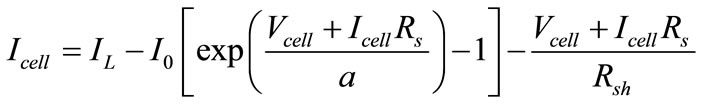
The DC part may be characterized by the I-V relationship [4,14]:
 (1)
(1)
Icell and Vcell are the current and the voltage of the PV cell, respectively. Given the meteorological parameters, the I-V curve can be determined uniquely. There are five parameters: the light current IL, the diode reverse saturation current I0, the series resistance Rs, the shunt resistance Rsh, and the modified ideality factor a. These pa-
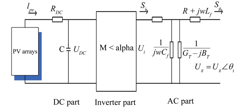
Figure 1. PV structure.
rameters depend on solar irradiance, the cell surface, and temperature.
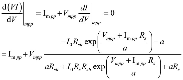
The differential of PV cell power to PV cell voltage is zero at the maximum power point (MPP), so the voltage Vmpp and current Impp at MPP can be solved by nonlinear Equations (1) and (2),
 (2)
(2)
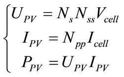
The PV module is composed of PV cells in series, and PV modules in series-parallel connection can form the PV array. The voltage UPV, the current IPV and the power PPV of the PV array can be calculated by (3), in which Ns is the series number of PV cell in a PV module, Nss is the series number of PV modules, and Npp is the parallel number of PV module strands [4]. Thus,
 (3)
(3)
The three-phase half-bridge inverter and SPWM are applied in the inverter part model. The fundamental wave voltage of phase-a is shown in Equation (4). The voltages of phase-b and phase-c are equal to that of phase-a, and they have a phase angle shift of 120˚ among them,
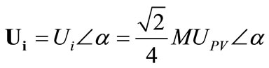 (4)
(4)
Based on the principle of instantaneous power balance, the real power exported by inversion part is equal to the DC power under the steady-state operation
Pi = PPV (5)
From Figure 1, the following power equations can be written,
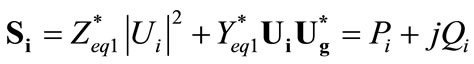 (6)
(6)
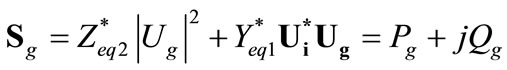 (7)
(7)
where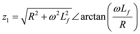 ,
,  ,
,  ,
,  ,
,  ,
,  ,
,  ,
,  ,
,  ,
,  , the superscript * means complex conjugate.
Thus, Equation (6)-(7) are included into the power flow solution in order to take into account the photovoltaic generation.
3. Wind Farm (WF) Modeling
Wind turbines (WTs) can either operate at fixed speed or variable speed. For a fixed speed wind turbine the generator is directly connected to the electrical grid. For a variable speed wind turbine the generator is controlled by power electronic equipment. There are several reasons for using variable-speed operation of wind turbines; among those are possibilities to reduce stresses of the mechanical structure, acoustic noise reduction, and the possibility to control active and reactive power [15,16]. Most of the major wind turbine manufacturers are developing new larger wind turbines in the 7-to-10-MW range [17,18]. These large wind turbines are all based on variable-speed operation with pitch control using a direct driven synchronous generator (without gearbox) or a doubly-fed induction generator (DFIG).
Fixed-speed induction generators with stall control are regarded as unfeasible for these large wind turbines [16]. Today, doubly-fed induction generators are commonly used by the wind turbine industry for larger wind turbines [19].
The major advantage of the doubly-fed induction generator, which has made it popular, is that the power electronic equipment only has to handle a fraction (20% - 30%) of the total system power [20,21]. This means that the losses in the power electronic equipment can be reduced in comparison to power electronic equipment that has to handle the total system power as for a direct-driven synchronous generator, apart from the cost saving of using a smaller converter.
Due to the fluctuation and intermittence of the wind power, large scale grid integration may result in an impact on the power system stable operation. Therefore, along with the enlargement of capacity of wind generators and the scale of wind farms, it is relevant to study the effect on the power system after large-scale grid integration. The power flow calculation is the basis of analyzing the influence of large scale integration, especially the basis of research foundation for power networks’ steady-state operation as well as its analysis.
When calculating the power flow including offshore wind power farms, we should take the steady-state mathematical model into consideration, extend it into the systematic equations, and then solve it with simultaneous equations. The equivalent circuit of asynchronous generators and the relationship of power transmission are shown in Figure 2. The wind is turned into mechanical energy by wind generators. The rotor’s power of an asynchronous generator is the power on the variable resistor r2 (1-s)/s of the equivalent circuit, where s is the generator’s slip ratio. The power PΩ subtracts the copper loss Pcu2, iron loss PFe and the stator copper loss Pcu1 is the power Pe of the power network. In Figure 2, xm and rm are, respectively, the excitation reactance and resistance; x1 and r1 are the stator’s reactance and resistance; x2 and r2 are the rotor’s reactance and resistance. In Figure 2, the stator resistance r1 and core losses PFe are neglected, due to xm ![]() x1. The excitation branch can be moved to the first end of the circuit, we got a simplified equivalent circuit of induction generator, Figure 3 [22-26].
x1. The excitation branch can be moved to the first end of the circuit, we got a simplified equivalent circuit of induction generator, Figure 3 [22-26].
The wind turbine generator (WTG) is designed to start to generate power at the cut-in speed vci and shut down for safety at the cut-out speed vco. Rated power PN is generated when wind speed is between rated speed vN and cut-out speed vco. There is a linear relationship between output power and wind speed when wind speed is between the cut-in speed vci and the rated speed vN [24,27]. The following equation is the mathematical expression for the power curve. The output power P corresponding to a given wind speed v can be obtained,
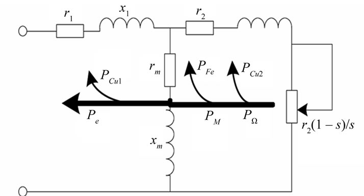
Figure 2. Equivalent circuit of WTG.
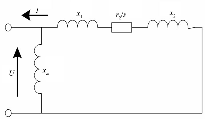
Figure 3. Simplified equivalent of WTG.
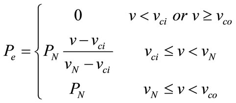 (8)
(8)
Hence, the power injected into the power system Pe is equal to electromagnetic power PM, which is the electric power on resistance r2/s. From Figure 3,
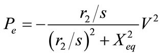 (9)
(9)
 (10)
(10)
where Xeq = x1 + x2.
From (9), the following equations can be written,
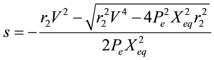 (11)
(11)
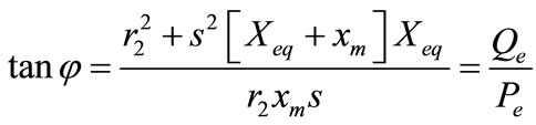
The relationship between the reactive power and active power of induction generator is derived from (10),
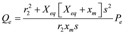 (12)
(12)
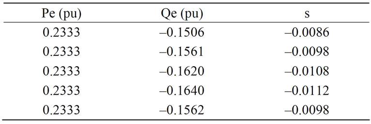
In this paper, the wind velocity v is assumed known, so that, through Equation (8) the electrical power is calculated. Then, the slip ratio s is evaluated by (11), assuming voltage V, which will be updated according to the power flow calculations, until convergence is attained. At each iteration, the required reactive power Qe is updated by Equation (12). In this method of calculation the offshore wind power farm is taken into account as a PQ bus.
4. Simulations
In this section, results showing the impact that PV and WF have over operative parameters when they are embedded into a test power system, Figure 4 [28], are presented. The following assumptions were taken into account: 1) There are twelve sites where to allocate PVs, from which just six must be elected; 2) There are nine sites where to allocate WFs, from which just five must be selected. The possible sites to allocate PVs are buses: {15 18 19 23 24 26 29 32 33 34 37 38}. Similarly, the possible sites to allocate WFs are buses: {11 13 16 17 21 28 31 35 39}. It is noteworthy that the abovementioned sites are elected arbitrarily; that is, without any special criterion, just with the purpose of assessing the renewable generation impact over the test power system’s operative condition. There are not generating buses in both lists. Likewise, the quantity of PVs and WFs is arbitrary. However, in this case, a limited budget is assumed,
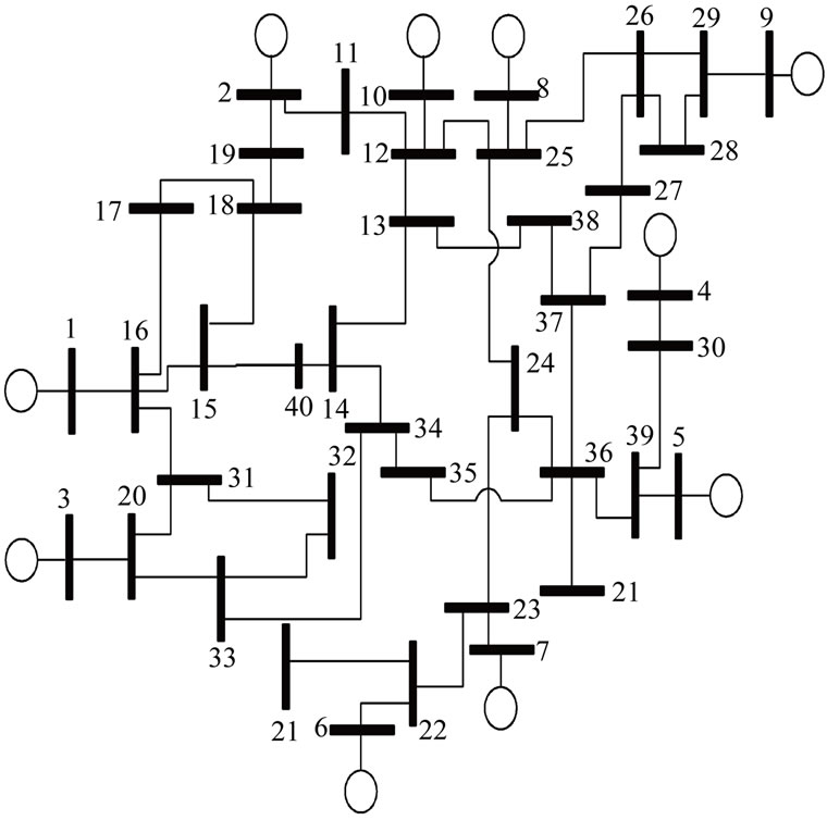
Figure 4. 39-Buses, 10-generators test system.
which not allows to build all possible facilities. Simulations are carried out in the following order: 1) Case 1: install six PVs facilities; 2) Case 2: install five WFs facilities; 3) Case 3: install six PVs and five WFs facilities. In all cases, independently of the allocation, the same capacity for PVs is assumed, likewise for WFs. Tables 1 and 2 summarize the relevant parameters for PVs and WFs, respectively [4,23]. It is assumed that PVs and WFs stations are connected to the grid through a transformer with 7% of reactance.
4.1. Methodology
In this paper, the impact of embedding renewable generation is assessed through a multi-objective optimization formulation; mono-objective formulations have been presented lately [29]. The decision variables are the PVs and WFs allocations. Three objective functions are taken into account: 1) System’s active losses; 2) System’s reactive losses; 3) The improvement of the load buses’ L-index [30]. This problem may be expressed as follows,
min f1 (active losses):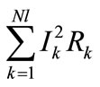 (13)
(13)
min f2 (reactive losses)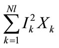 (14)
(14)
min f3 = Lindex (15)
subject to
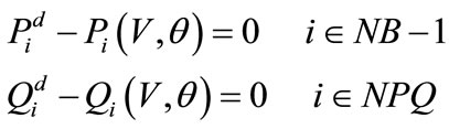 (16)
(16)
where Ik, Rk, and Xk are the absolute value of the current
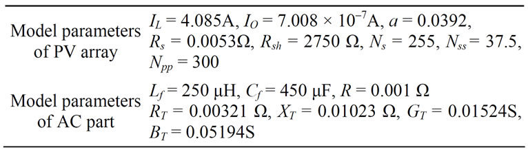
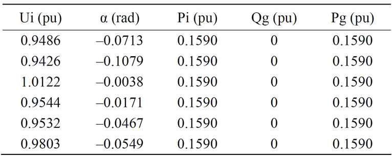
Table 1. PV power station’s parameters.
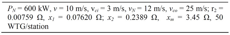
Table 2. WTG parameters.
through the k-th transmission line, its resistance and reactance, respectively; Lindex is the worst load buses’ L-index; Nl represents the number of transmission lines; NB is the system’s buses set; NPQ is the PQ-buses set. Eqution (16) represents the load flow equations. V is the bus voltage magnitude and θ its phase; Pid, Qid are the active and reactive power demand at the i-th bus, respectively.
The reason to use the L-index is due to it is an approximate measure about the system’s closeness to voltage collapse. Its calculation is based on load flow analysis, and its value ranges from 0 (no load condition) to 1 (voltage collapse). The bus with the highest L-index value will be the most vulnerable bus in the system. The L-index for the j-th bus is calculated by the expression,
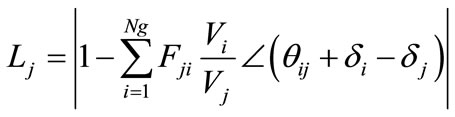 (17)
(17)
where Vi, Vj are the i-th and j-th generators’ voltage magnitude, θij is phase angle of the term Fji, δi, δj are the voltage phase angle of i-th and j-th generating unit [30].
In order to solve the problem formulated by Equation (13)-(16), the Non-dominated Sorted Genetic Algorithm (NSGA-II) has been used. Srinivas and Deb [31,32] propose the NSGA, which is based on several layers of individuals’ classifications. Before the selection is performed, the population is ranked on the basis of non-domination. All non-dominated individuals are classified into one category, with a dummy fitness value, which is proportional to the population size, to provide an equal reproductive potential for these individuals. To maintain the population’s diversity, these classified individuals are associated with their dummy fitness values. Then this group of classified individuals is ignored and another layer of non-dominated individuals is considered. The process continues until all individuals in the population are classified. Since individuals in the first front have the maximum fitness value, they always get more copies than the rest of the population. This allows searching for non-dominated regions, and results in quick convergence. Figure 5 depicts a flowchart to solve the proposed strategy. In this paper, the number of generations are MNG = 20, and the population size is POP = 20.
Since the sites where to allocate renewable energy has a discrete nature, strictly, the optimization problem must be formulated as an integer nonlinear problem. However, in this paper variables are continuous type and they are rounded to the nearest integer value. Thus, the ranges of such discrete variables are within ximax and ximin (maximum and minimum values of the i-th discrete control variable xi), which can take Ni number of different discrete values within its range.
4.2. Results
According to the proposed methodology, the PVs (WFs) allocation and their parameters become
• Case 1: PVs installed in {18 19 24 32 34 38}
• Case 2: WFs installed in {11 13 16 17 21}
• Case 3: PVs installed in {15 18 26 33 34 38}

WFs installed in {11 13 16 17 31}
Table 3 summarizes the results of active and reactive power losses and the L-index, when the PVs and WFs stations are allocated in the abovementioned buses. Respect to the active power losses, the variations are mini-
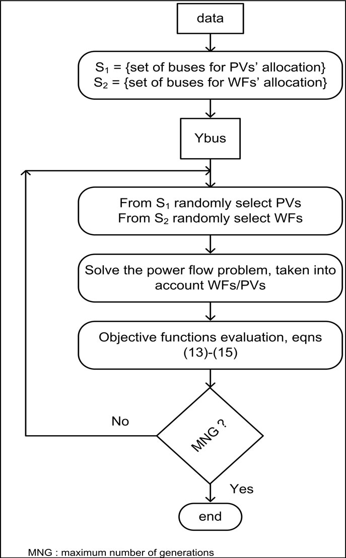
Figure 5. flowchart to solve the optimization problem.
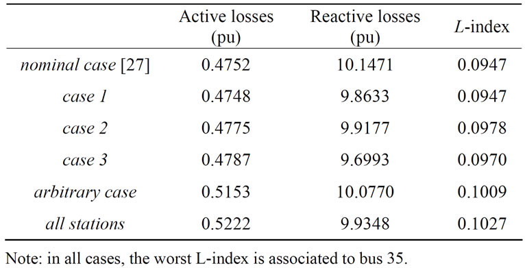
Table 3. Objective function’s value.
mal, respect to the nominal case (without any renewable source). The main reason is due to the fact that practically all power stemming from the renewable sources is consumed right there. That is, the amount of generated power is just a fraction of the total load, and it is consumed on the site. Larger variations are attained if larger resources are available, and consequently larger power stations can be built.
The reactive power losses undergo more variation respect to the nominal case, mainly due to the fact that the wind farms require reactive support. In this paper, it is assumed that no reactive resources are available where the WFs stations are allocated. This would improve the power losses, however, at the expenses of additional financial budget.
Finally, the L-index remains almost unaltered under different conditions, since this test system is robust, from the voltage stability point of view. This index could undergo notorious variations if the amount of injected power were substantially greater. Nevertheless, as in the above paragraph, the reactive power requirements modify the L-index as can be noticed in cases 2 and 3. In all cases, bus 35 exhibits the worst L-index.
As a mean to highlight the optimized results, an arbitrary allocation of stations is simulated. For example: 1) PV stations sited in buses {19 23 24 29 32 37}; 2) WF stations sited in {21 28 31 35 39}. Under this conditions, in row sixth of Table 3, the objective functions are summarized. It is noteworthy that worst results are obtained, respect to the optimized case 3.
If all stations could be built (both PVs and WFs), the objective functions would be as the seventh row in Table 3 shows. In this case, there are notorious variations mainly due to the reactive power requirements at the WFs stations. These, account for the followingReactive injection at the WFs facilities: {–0.1507 –0.1565 –0.1624 –0.1643 –0.1565 –0.1525 –0.1619 –0.1618 –0.1562}
These reactive requirements, modifies the L-index too. Figure 6 depicts a comparison among the reactive powerdelivered by the ten conventional generating units for the nominal case, case 2, and if all facilities are built. The difference is now notorious.
Figure 7 shows the active power flow through transmission lines for case 1 and if all facilities were built.
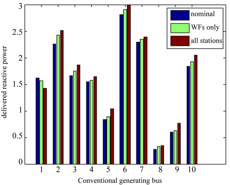
Figure 6. Reactive power delivered by the conventional generators.
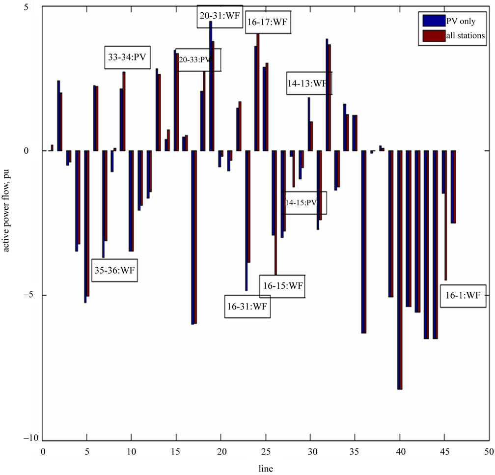
Figure 7. Active power flow through transmission lines.
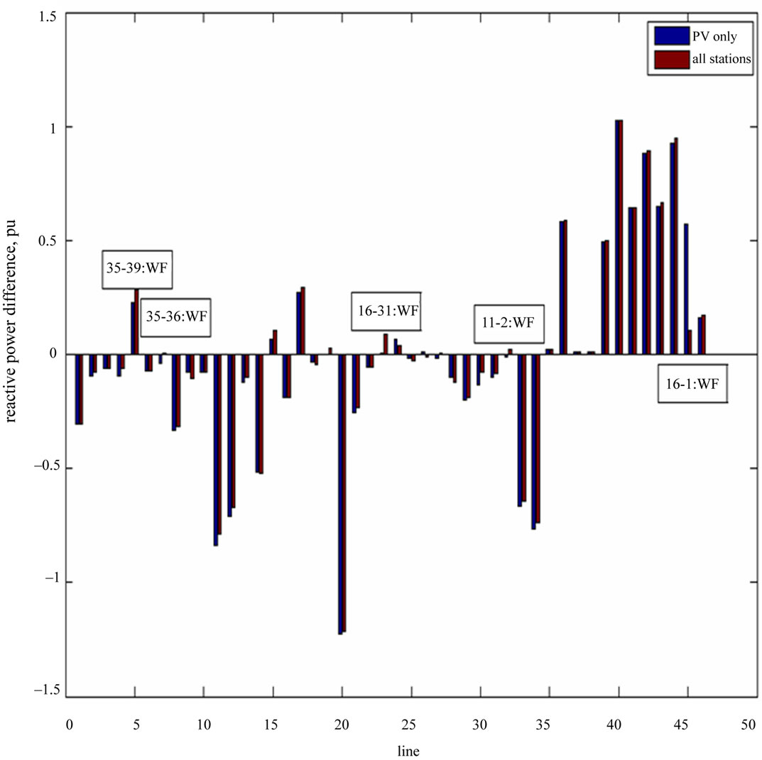
Figure 8. Sending and receiving difference in reactive power.
The lines where there is a notorious difference are noticed. Likewise, Figure 8 displays the difference between the sending and receiving reactive power flow in transmission lines, for the two aforesaid cases; the main differences are noticed too. In both cases, the main differences are associated to some of the PVs or WFs stations.
Thus, nowadays, it is essential that power flow programs include different types of renewable energy models, since these classes of energies have widespread use. Overall at the planning stage, special care should be paid to the reactive power management, since, beyond doubt, it is a relevant issue to be taken into account. In this paper, one class of such models is presented. However, there exist a variety of propositions that could be better adapted to the specific local industry necessities [4,9,13, 22,24-26].
4.3. Costs
Strictly, within the proposed formulation, Equation (13)-(14), costs must be taken into account. A way to do it, may be as a fourth objective function,
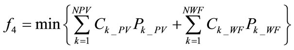 (18)
(18)
where NPV (NWF) is the number of PV (WF) stations to be installed; Ck_PV (Ck_WF) is the cost of the k-th photovoltaic (wind) facility per Watt; Pk_PV (Pk_WF) is the output power in the k-th photovoltaic (wind) station. In this paper, such function are not included because of the related public information widely varies among countries and among manufacturers. However, this information can be added straightforwardly into the proposed formulation.
5. Conclusions
Due to the wider use of renewable energy, it is quite important to take it into account when steady state power flow studies are carried out. This paper summarizes modeling of photovoltaic and wind farm stations to be embedded into the conventional power flow formulation. It is assumed that there exist a reduced number of such stations to be added into the power system. Their allocation is decided based on a multiobjective optimization strategy. The inclusion of costs’ stations into the formulation is straightforward. Results show that a careful reactive power management is required in grids where there are important contributions of wind farm stations, since they represent reactive loads.
6. Acknowledgements
Author thanks CFE-CONACyT under grant 88160.
REFERENCES
- R. Strzelecki and G. Benysek, “Power Electronics in Smart Electrical Energy Networks,” Springer, London, 2008. doi:org/10.1007/978-1-84800-318-7
- A. Keyhani, M. N. Marwali and M. Dai, “Integration of Green and Renewable Energy in Electric Power Systems,” John Wiley and Sons Inc., Hoboken, 2010.
- C. W. Gellings, “The Smart Grid. Enabling Energy Efficiency and Demand Response,” The Fairmont Press Inc., Lilburn, 2009.
- Y.-B. Wang, C.-S. Wu, H. Liao and H.-H. Xu, “SteadyState Model and Power Flow Analysis of Grid-Connected Photovoltaic Power System,” ICIT 2008. IEEE International Conference on Industrial Technology, Chengdu, 21-24 April 2008.
- J. D. Mondol, Y. G. Yohanis and B. Norton, “Comparison of Measured and Predicted Long Term Performance of Grid a Connected Photovoltaic System,” Energy Conversion and Management, vol. 48, 2007, pp. 1065-1080. doi:org/10.1016/j.enconman.2006.10.021
- M. Cucumo, A. D. Rosa, V. Ferraro, D. Kaliakatsos and V. Marinelli, “Performance Analysis of a 3 kW GridConnected Photovoltaic Plant,” Renewable Energy, Vol. 31, 2006, pp. 1129-1138. doi:org/10.1016/j.renene.2005.06.005
- R. González, J. López, P. Sanchis and L. Marroyo, “Transformerless Inverter for Single-Phase Photovoltaic Systems,” IEEE Transaction on power electronics, Vol. 22, 2007, pp. 693-697.
- T. F. Wu, C. L. Shen, H. S. Nein and G. F. Li, “A 1ø 3 W Inverter with Grid Connection and Active Power Filtering Based on Nonlinear Programming and Fast-Zero-Phase Detection Algorithm,” IEEE Transactions on Power Electronics, Vol. 20, 2005, pp. 218-226. doi:org/10.1109/TPEL.2004.839786
- M. Nagao and K. Harada, “Power Flow of Photovoltaic System Using Buck-Boost PWM Power Inverter,” Proceeding of 1997 International Conference on Power Electronics and Drive Systems, Tehran, 3-5 November 1997.
- S. Saha and V. P. Sundarsingh, “Novel Grid-Connected Photo Voltaic Inverter,” IEE proceeding on Generation, Transmission and Distribution, Vol. 143, 1996, pp. 219- 224. doi.org/10.1049/ip-gtd:19960054
- C. Rodriguez and G. A. J. Amaratunga, “Dynamic Stability of Grid Connected Photovoltaic Systems,” 2004 IEEE Power Engineering Society General Meeting, pp. 2193- 2199, Denver, 6-10 June 2004.
- B. Yang, W. L. Y. Zhao and X. He, “Design and Analysis of a Grid-Connected Photovoltaic Power System,” IEEE Trans on Power Electronics, Vol. 25, No. 4, April 2010, pp. 992-1000.
- B. Kroposki, “Power System Studies and Modeling PV Inverters,” Utility/Lab Workshop on PV Technology and Systems, Tempe, November 8-9, 2010.
- W. de Soto, S. A. Klein and W. A. Beckman, “Improvement and Validation of a Model for Photovoltaic Array Performance,” Solar Energy, Vol. 80, 2006, pp. 78-88. doi:org/10.1016/j.solener.2005.06.010
- A. Petersson, “Analysis, Modeling and Control of Doubly-Fed Induction Generators for Wind Turbines,” Ph.D. Dissertation, Division of Electric Power Engineering, Department of Energy and Environment, Chalmers University of Technology, Goteborg, 2005.
- T. Burton, D. Sharpe, N. Jenkins and E. Bossanyi, “Wind Energy Handbook,” John Wiley & Sons Inc., Hoboken, 2001. doi:org/10.1002/0470846062
- C. Ksenia, S. Riffat and J. Zhu, “An Overview of Renewable Energy Policies and Regulations in People’s Republic of China,” Proceedings of ICRM 2010, 5th International Conference on Responsive Green Manufacturing, University of Nottingham, Ningbo, 11-13 January 2010.
- H. S. Kim and D. D. Lu, “Wind Energy Conversion System from Electrical Perspective—A Survey,” Smart Grid and Renewable Energy, Vol. 1, 2010, pp. 119-131. doi:org/10.4236/sgre.2008.13017
- GE Wind Energy. (2005, Jan.) 3.6 s offshore wind turbine. Brochure. http://www.gepower.com/prod serv/products/wind turbines/en/ downloads/ge 36 brochure.pdf
- L. Xu and C. Wei, “Torque and Reactive Power Control of a Doubly Fed Induction Machine by Position Sensorless Scheme,” IEEE Transactions on Industry Applications, Vol. 31, No. 3, 1995, pp. 636-642. doi:org/10.1109/28.382126
- L. Morel, H. Godfroid, A. Mirzaian and J. Kauffmann, “Double-Fed Induction Machine: Converter Optimisation and Field Oriented Control without Position Sensor,” IEE Proceedings Electric Power Applications, Vol. 145, No. 4, July 1998, pp. 360-368. doi:org/10.1049/ip-epa:19981982
- Z. Wei, W. Zhinong and S. Guoqiang, “Power Flow Calculation for Power System Including Offshore Wind Farm,” International Conference on Sustainable Power Generation and Supply, 2009, Nanjing, 6-7 April 2009.
- J. Kilter, M. Landsberg, I. Palu and O. Tšernobrovkin, “Verification of Wind Parks and their Integration into Small-Interconnected Power System,” IEEE Bucharest Power Tech Conference, Bucharest, 28 June-2 July 2009.
- X. Han, M. Mu and W. Qin, “Reliability Assessment of Power System Containing Wind Farm Based on SteadyState Power Flow,” 11th International Conference on Probabilistic Methods Applied to Power Systems (PMAPS 2010), Singapore, 14-17 June 2010.
- A. E. Feijoo and J. Cidras, “Modeling of Wind Farms in the Load Flow Analysis,” IEEE Transactions on Power Systems, Vol. 15, No. 1, 2000, pp. 110-115. doi:org/10.1109/59.852108
- A. E. Feijoo, J. Cidras and J. L. G. Dornelas, “Wind Speed Simulation in Wind Farms For Steady-State Security Assessment of Electrical Power Systems,” IEEE Transactions on Energy Conversion, Vol. 14, No. 4, December 1999, pp. 1582-1588.
- M. R. Haghifam and M. Omidvar, “Wind Farm Modeling in Reliability Assessment of Power System,” International Conference on Probabilistic Methods Applied to Power Systems, PMAPS 2006, 11-15 June 2006, pp. 1-5.
- K. R. Padiyar, “Power System Dynamics. Stability and Control,” John Wiley and Sons (Asia), 1996.
- A. M. El-Zonkoly, “Optimal Placement of Multi DG Units Including Different Load Models Using PSO,” Smart Grid and Renewable Energy, Vol. 1, 2010, pp. 160 -171. doi:org/10.4236/sgre.2008.13021
- P. Kessel and H. Glavitsch, “Estimating the Voltage Stability of a Power System,” IEEE Transactions on Power Delivery, Vol. 1, No. 3, 1986, pp. 346-354. doi:org/10.1109/TPWRD.1986.4308013
- N. Srinivas and K. Deb, “Multiobjective Function Optimization Using Non-dominated Sorting Genetic Algorithms,” Evolutionary Computation, Vol. 2, No. 3, 1994, pp. 221-248. doi:org/10.1162/evco.1994.2.3.221
- K. Deb, A. Pratap, S. Agarwal and T. Meyarivan, “A Fast and Elitist Multi-objective Genetic Algorithm: NSGA-II,” IEEE Transactions on Evolutionary Computation, Vol. 6, No. 2, 2002, pp. 182-197. doi:org/10.1109/4235.996017