Journal of Water Resource and Protection
Vol. 2 No. 2 (2010) , Article ID: 1311 , 11 pages DOI:10.4236/jwarp.2010.22017
Estimation of Evapotranspiration from Faber Fir Forest Ecosystem in the Eastern Tibetan Plateau of China Using SHAW Model
1Key Laboratory of Ecosystem Network Observation and Modeling, Institute of Geographical Sciences and Natural Resources Research, Chinese Academy of Sciences, Beijing, China
2Graduate University of the Chinese Academy of Sciences, Beijing, China
3Integrated Water and Hazards Management International Centre for Integrated Mountain Development (ICIMOD) Kathmandu, Nepal
E-mail: yinzf@igsnrr.ac.cn, houyang@icimod.org, xuxingl@hotmail.com, zhoucp@igsnrr.ac.cn, zhangf@igsnrr.ac.cn, shaob@igsnrr.ac.cn
Received November 15, 2009; revised December 18, 2009; accepted December 24, 2009
Keywords: evapotranspiration, faber fir forest, Tibetan Plateau, SHAW
ABSTRACT
Understanding the hydrological processes of forest ecosystems in Tibetan Plateau is crucial for protecting water resources and the environment, especially considering that evapotranspiration is the most dominant hydrologic process in most forest systems. SHAW, as a physically based, hydrological model, provides a useful tool for understanding and analyzing evapotranspiration processes. Using the measured data of a faber fir forest ecosystem in eastern Tibetan Plateau, this paper assessed the model performance in simulating evapotranspiration and variability and transferability of the model parameters. Comparison of the simulated results by SHAW to the measured data showed that SHAW performed satisfactorily. Based on analyzing the simulated results by the calibrated and validated SHAW, some ET characteristics of faber fir forest ecosystem in the eastern Tibetan Plateau were found: 1) Daily plant transpiration is low, and daily ET mainly comes from surface evaporation including canopy, litter and soil evaporation. Peak ET rate was approximately 4mm/day, occurring around late July. 2) Solar radiation is the most important factor accounting for daily ET variation, while air temperature is the secondary, wind speed and air relative humidity are minor and soil water storage is the least important among all the related factors. 3) The ratio of annual ET to precipitation for the faber fir forest ecosystem in eastern Tibetan Plateau is low (18%) compared with the other forest ecosystems owing to high-elevation, high atmospheric humidity and low annual temperature.
1. Introduction
The transport of water in forest ecosystems is important because of concerns about effects of climate on vegetation and about influences of forest management on floods, seasonal low flows, and water and soil loss. Meanwhile, hydrological processes are difficult to study because they are influenced by a myriad of biophysical factors. Forest hydrology, an important science addressing the relationship between forests and hydrology, has received significant attention globally.
Evapotranspiration is the most important factor in the forest hydrological cycle that links other processes (such as runoff, deep percolation et al.) [1]. However, there is a logical paradox between evapotranspiration, humidity and temperature in forest when explaining some observations, because of insufficient understanding of forest hydrological processes due to the complex structure of forests [2,3]. Field studies and complementary modeling programs have increased our understanding of the processes controlling water transport in forest ecosystems (e.g.,[3]).Physically based models have greatly increased our understanding of the complex interactions between hydrologic processes and vegetation.
It is particularly important to increase our understanding about the water transport mechanisms of forest ecosystems in regions such as the Tibetan Plateau, that are sensitive to climate change and whose variability could influence Northern hemispheric or global ecosystems [4]. Dark coniferous forest is the main body of forest vegetation in the alpine region of eastern edge of Tibetan Plateau and the most important vegetation type for water conservation in the upper reaches of the Yangtze River. Among that, faber fir (Abies fabri) is the most typical. So, this paper selected the faber fir forest ecosystem in eastern Tibetan Plateau to study its evapotranspiration processes, the particularly critical hydrological process of forest ecosystems, using a physically based numerical model.
Existing Soil-Vegetation-Atmosphere Transfer (SVAT) models simulate a number of interrelated mass and energy transfer processes through layered soil-vegetationatmosphere systems [5–7].
Among the SVAT models, Simultaneous Heat and Water (SHAW) model is the most representative; it is a one dimensional hydrologic model that integrates the coupled transport of water and energy through a soil-vegetation-atmosphere systems into a simultaneous solution [6,8,9]. The model was validated and applied over a variety of vegetation covers under some different climate conditions such as semiarid and arid cropland and rangeland, as well as humid forests. Many aspects of the model have been tested, including the effects of vegetation on soil temperature and moisture [10], snowmelt [11,12], soil freezing [9,13], evapotranspiration and surface energy budgets [6], and soil deep percolation [14]. To date, the SHAW model has not been tested in alpine forest although it has been tested in the humid forest of U.S. Pacific Northwest [15].
The objectives of this paper are: 1) to determine the parameters of the SHAW model for application in the dark coniferous forest in alpine region of Tibetan Plateau; 2) to validate the key hydrologic processes and state variables simulated by the model, including evapotranspiration and soil water content; and 3) to quantify the annual and daily evapotranspiration; and 4) to illuminate the factors influencing evapotranspiration.
2. Materials and Methods
2.1. Materials
2.1.1. Site Description
Tibetan Plateau is in the southwest of China (Figure 1). The area of Tibetan Plateau is about 2.5 million km2, forest ecosystem mainly distributes over southeast of the Plateau. This study was conducted at Gongga Mountain Alpine Ecosystem Observation and Experiment Station of Chinese Academy of Sciences, located within the dark coniferous forest, in alpine region of eastern edge of Tibetan Plateau. The site is located at an elevation of 3060 m, on the gently eastern slope of Gongga Mountain in the Huangbengliu Valley, at 29° 34′N latitude, 102° 0′E longitude.
Climate at the site is characterized by wet, cool summers and dry, moderate winters, with an average annual precipitation of 1932 mm (measured from 1988 to 2003). About 80% of the precipitation occurs May through October, the mean annual rainy days is above 260. Mean annual air temperature is 4.2℃, with the mean monthly maximum of 14.0℃ occurring in July, and the mean monthly minimum of -1.7℃ occurring in January.
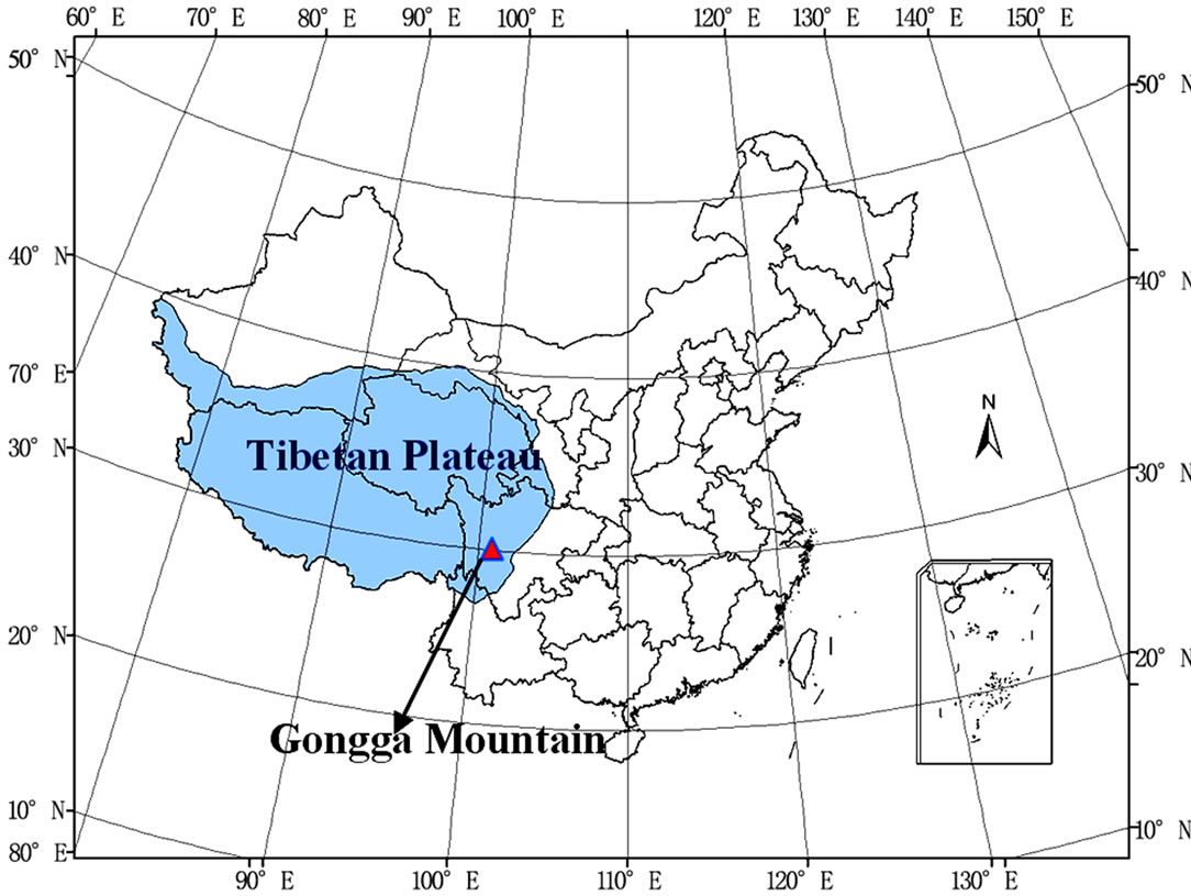
Figure 1. The locations of the Tibetan Plateau and Gongga Mountain.
Dominant specie at the site is faber fir, with most individuals exceeding 70 year in age and approximately 15m in height. The understory of faber fir forest is comprised of broadleaf arbor, shrub and herbage. The broadleaf arbor is composed of coarse-bark birch (Betula utilis D. Don) and big-leaf poplar (Populus lasiocarpa Ol iv.). The shrub includes sims azalea (Rhododendron simsii Planch) and sheepberry (Viburnum spp.). The canopies of broadleaf arbor and shrub under of faber fir are interlaced and averagely 5m in height. The herbage comprises cuckoopint (Trillium tschonoskii) and wintergreen (Pyrola calliantha H. Andr.). In growing season, the herbage is averagely 30cm in height. A high diversity of nonvascular plants is present in the soil or residue surface, dominated by lichens and bryophytes.
Soil at the site is classified as mountain dark brown soil, and consists of loamy sands and sandy loams characterized by low bulk densities and high porosities. The soil is thin, and gravels are present below 40cm, owing to the parent materials originating from slope deposit of debris flow. The organic matter content is high in the top soil layer. Litters are in the semi-decomposed state, with a thickness of approximately 8cm [3].
2.1.2. Data Measurements
1) Weather and gradient microclimate measurements The AMRS-I automated weather station located at an elevation of 3060m in eastern slope of Gongga Mountain, to measure total radiation, net radiation, air temperature, wind velocity, rainfall, humidity, soil heat flux and soil temperature. 30-m iron tower installed was used as an instrument platform for gradient microclimate measurements (model MAOS-1) in the forest. Air temperature and relative humidity were measured using ventilated psychrometer sensors (model HTF22), the sensors accuracy are 0.1℃ and 0.1hPa respectively. The heights of the measurements were 1.5m, 10m, 15m and 18m above the ground. Soil temperature at 5cm, 10cm, 15cm, 20cm, 40cm, 70cm and 100cm depth were measured with platinum resistance temperature sensors (model HBW22B). These microclimate data were collected by an automated collecting system hourly.
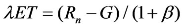
2) Bowen ratio-energy balance method of determining ET The Bowen ratio [16] and the energy balance equation are the basis for the Bowen ratio-energy balance method of determining ET using microclimate and soil heat measurements [17,18]. Based on the gradient microclimate measurements at 15m and 18m, the evapotranspiration from the forest could be calculated using Bowen ratio energy balance method. The latent heat flux can be estimated by Bowen ratio energy balance method as follows:
 (1)
(1)
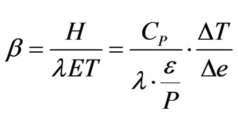
where λET is the latent heat flux (W/m2), λ is the heat of water vaporization (J/kg), vaporization (J/kg), ET the evapotranspiration (mm), Rn the net radiation (W/m2), and G is the ground heat flux (W/m2). Bowen ratio β is defined as follows:
 (2)
(2)
where ΔΤ and Δе are the temperature (℃) and vapor pressure difference (kPa) between the two measurement levels, respectively; Cp is the constant-pressure specific heat, usually, Cp=1005J·kg-1·K-1, ε is the ratio of the molecular weight of water to that of dry air(ε=0.622), P is the atmospheric pressure. Then the evapotranspiration can be calculated from Equations (1) and (2).
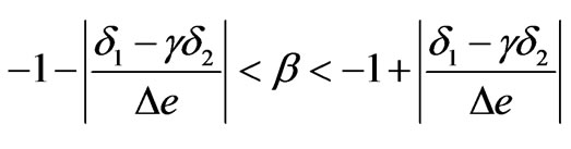
In this study, Rn and G in equation (1) were obtained from AMRS-Ⅰautomated weather station. It is noticeable that Bowen ratio β was at the order of -1 sometimes during nighttime or precipitation when atmosphere was instable. While Bowen ratio β is around the value of -1, Equation (1) is abnormal, so some authors discussed the standard for judging invalid β [19–21]. In this paper, we used the method providing by Perez et al. [21] to exclude the invalid β, which considering the accuracy of temperature and humidity measurements and the water vapor press difference adequately. The invalid β value range was determined as follows:
 (3)
(3)
where δ1 (kPa) and δ2 (K) are the measurement accuracy for humidity and temperature.
3) Soil water content measurements A long-term observation plot of the Chinese Ecosystem Research Network was located near the weather station. Volumetric soil water content was measured at 10cm, 30cm, 40cm, 60cm and 100cm depths at 5 days interval using HH2 handheld moisture meter (Delta-T Devices Ltd. England) at five different sites of the plot. The accuracy for measurement is 0.1% moisture.
4) Leaf area index measurement Leaf area index were measured using digital plant canopy imager (CI-110, CID Ltd., U.S.A.) in 2005. Leaf area index of the faber fir forest ecosystem is given in Table 1.
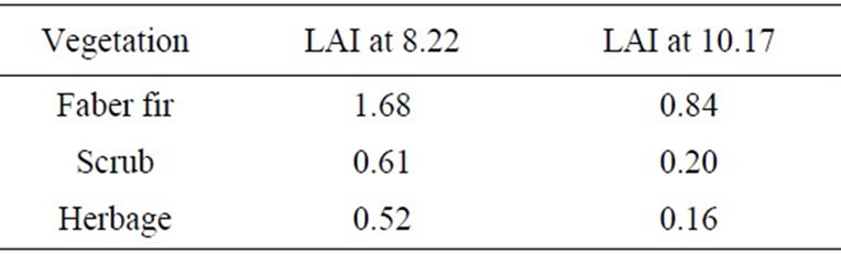
Table 1. Leaf area index for vegetation of the site.
2.2. Methods
2.2.1. Model Description
The SHAW model was originally established in 1989 [8] and a vegetation canopy was added in 1991 [22]. It simulates a vertical, one-dimensional system composed of a vegetation canopy, snow cover (if present), residue and soil profile. A conceptual diagram of the model structure is shown in Figure 2. The model integrates the detailed physics of interrelated mass and energy transfer through the multilayer system and includes the process of soil freezing and thawing. Daily or hourly predictions include evaporation, soil frost depth, snow depth, and soil profiles of temperature, water, ice, and solutes.
Boundary conditions are determined by routine weather variables above the canopy, including air temperature, wind velocity, air humidity, total radiation and precipitation, and soil water content and soil temperature at the lower boundary. The canopy can be separated into 10 layers and the soil profile can be divided into 50 layers at most. After computing flux at the upper boundary, the heat, liquid water, and vapor flux between layers are computed. Heat and water flux through the system are calculated simultaneously using implicit finite-difference equations that are solved iteratively using a Newton-Raphson procedure [23]. The model can simulate heat and water transfer in canopies comprised of several different plant species (including standing dead material). Plant height, biomass, leaf area index, rooting depth, and leaf dimension are specified by the user. Details of the numerical implementation of the SHAW model are presented in [24,25], and [8]. According to the description of these literatures, the basic computation procedures applied in this paper are described in the following sections:
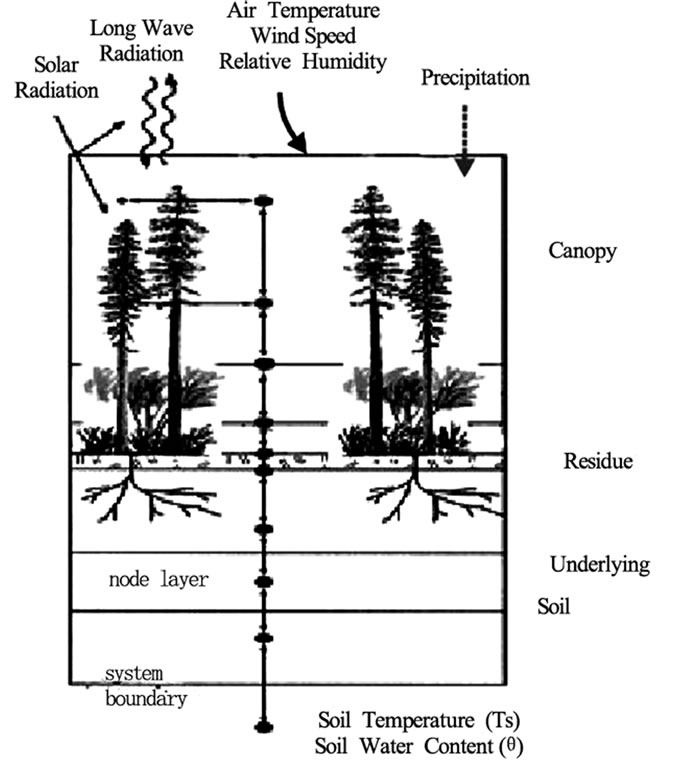
Figure 2. Conceptual diagram of SHAW model.
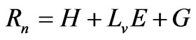
1) Energy and water fluxes at the upper boundary of the multilayer system The inputs of energy and water into the upper boundary are computed from the basic meteorological elements at the standard weather stations, including air temperature, wind speed, air humidity, total radiation and precipitation. Precipitation is the water input the upper boundary. The energy inputs are calculated with the energy balance equation:
 (4)
(4)
where  is net radiation (W m−2),
  is sensible heat flux (W m−2),
  is latent heat flux (W m−2),
  is subsurface conductive heat flux (W m−2),
  is evaporation latent heat (J kg−1) and E is the total evapotranspiration of the multilayer system (kg m−2 s−1). Among them net radiation is determined by the transmission of solar radiation and long-wave radiation the multilayer system. In the vegetation canopy, radiation transmission is calculated from leaf area index and leaf inclination, as described by Flerchinger et al. [6]. Leaf aledo is input to the model, and soil surface albedo is involved with surface water content. Long wave radiation is calculated from air temperature and daily mean cloud coverage estimated with measured solar radiation as described by Flerchinger et al. [12]. Sensible and latent heat flux at the upper boundary are computed from temperature and vapor gradients between the canopy-residue-soil surface and the atmosphere. Sensible heat flux is computed from [26]:
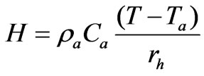 (5)
(5)
where ,
,  and
and  are the density (kg m-3), specific heat (J-1 kg-1) and temperature (℃) of air at the measurement reference height,
  is the temperature (℃) of the exchange surface, and
  is the resistance to surface heat transfer (s m-1) corrected for atmospheric stability. Latent heat flux is associated with transfer of water vapor from the exchange surface to the atmosphere, which is given by
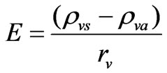 (6)
(6)
where  and
and  are vapor density (kg m-3) of the exchange surface and at the reference height and the resistance value for vapor transfer,
  is taken to be equal to
  .
.
The subsurface conductive heat flux is computed from Equation (4), which satisfies the whole balance of the energy fluxes in the multilayer system.
2) Plant transpiration Plant stomas are assumed to close if light or temperature conditions are not adequate for transpiration. If incoming solar radiation is less than 10 W m2, or if the air temperature Ta, is colder than a specified minimum air temperature, transpiration is set to zero and there is no vapor transfer from the canopy elements for the given plant species.
Transpiration within a canopy layer is determined assuming that soil-plant-atmosphere is a continuum. Water flow is computed assuming continuity in water potential throughout the plants, and can be computed at any point in the plant from
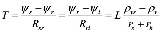 (7)
(7)
 is total transpiration rate (kg m-2s-1) for a given plant species;
 ,
, and
and  are the water potential (m) in layer of soil, roots and leaves, respectively; Rsr and Rrl are the resistance to water flow (m-3s kg-1 ) through the roots of soil layer and the leaves of canopy layer; L is leaf area index for the given species;
  is the vapor density (kg m-3) within the stomata cavities (assumed to be saturated vapor density);
  is the vapor density of the air within canopy layer;
  is stomata resistance per unit of leaf area index (s m-1);
  is resistance to convective transfer within the layer per unit of leaf area index(s m-1).
Water flow within the plant is controlled mainly by changes of stomata resistance. Neglecting other effects, a simple equation relating stomata resistance to leaf water potential is
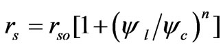 (8)
(8)
where  is stomata resistance (m s-1) with no water stress (assumed constant),
  is a critical leaf water potential (m) at which stomata resistance is twice its minimum value, and n is an empirical coefficient [23].
2.2.2. Determination of Model Parameters
The SHAW model is physically based and a number of physical parameters describing the site and the vegetation status are required. All original parameters were derived from measurements at the site where possible, or estimated from literature values. Some special parameters were adjusted during model calibration through sensitivity analysis.
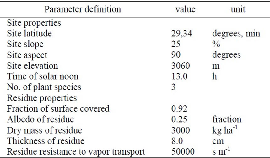
Table 2. Site parameters of SHAW model.
1) Site parameters The site parameters of Gongga Mountain faber fir forest for the SHAW model are listed in Table 2. Fraction of surface covered by residue and thickness of residue were estimated based on field survey. Residue albedo and resistance to vapor transport were the suggested value in user’s manual [25]. Dry mass of residue was derived from literature [27].
2) Vegetation parameters Three plant species were simulated in order to describe the vegetation characteristics in detail. It is noteworthy that the canopies of broadleaf arbor and shrub under of Faber fir were in the same height and interlaced, so they were taken as one plant specie and simply called scrub in this study. Similarly, cuckoopint and wintergreen were put together in herbage. The parameters of the three plant species are given in Table 3. Albedo of faber fir and scrub were estimated based on the albedo range of different vegetations listed by the literature [28]. The albedo of herbage was obtained from Cheng et al. [29]. The transpiration threshold values of three types of plant were determined according to the literature [28]. Minimum stomata resistance of the three types of plant was estimated from the data observed by Cheng et al. [29]. Resistance function exponent and critical leaf water potential for three types of plant were estimated on the basis of the suggested values in users’ manual [25] and model sensitivity analysis. Leaf resistance and root resistance for three types of plant were set based on the physiological principle indicated by Campbell [23] that roughly 1/3 of the resistance to water flow within plants is encountered within the leaves.
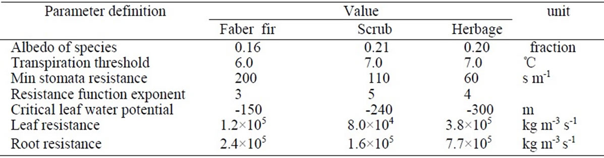
Table 3. Vegetation parameters of SHAW model.
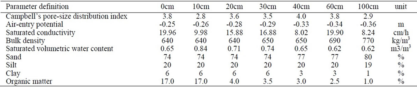
Table 4. Soil parameters of SHAW model.
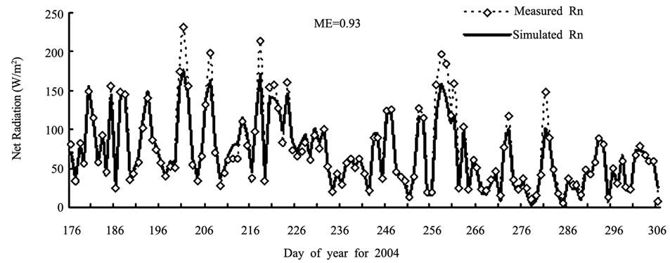
Figure 3. Simulated and measured net radiation for 2004.
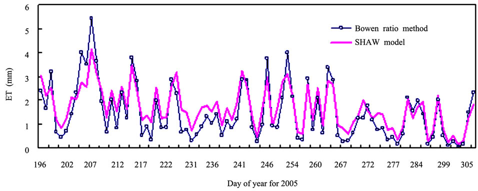
Figure 4. Simulated and measured daily evapotranspiration for 2005.
3) Soil parameters Based on soil characteristics and available measured data, soil profile was divided into 7 layers. The parameters for every soil layer are shown in Table 4. Bulk density, saturated conductivity, saturated volumetric water content, soil particle-size composition (sand, silt, clay) and organic matter were measured by Cheng et al. [3]. Campbell’s pore-size distribution index and air-entry potential were estimated according to the model recommended ranges [25].
4) Model Calibration Mass and energy dynamics were simulated for 2004 year to calibrate the model parameters. Firstly, the soil properties used in the model were optimized by comparing soil water content simulated to the measured data during the 2004 development period. Parameter adjustments were limited to the measured and estimated soil properties (specifically, saturated conductivity, air-entry potential and the pore size distribution index) to more accurately simulate the observed drainage trends. The final soil parameters are listed in Table 4. Then, the originally determined vegetation parameters were calibrated by comparing net radiation simulated to the measured data. Sensitivity analysis suggested that albedo values of plants were the main factors to decide net radiation. Through adjusting the faber fir albedo value from 0.14 to 0.16 and adjusting herbage albedo from 0.19 measured by Cheng et al. [29] to 0.20, the simulated net radiation attained the optimal values comparing the measured data. Finally vegetation parameters in Table 3 were determined. Figure 3 shows the simulated and measured net radiation for June to October of 2004. The model could simulate the net radiation trends quite well. The model efficiency (ME, defined in “5. Model validation”) for simulated net radiation during the 2004 development period was 0.93.
5) Model validation The parameters used in the 2004 simulations were subsequently applied without modification for 2005. The simulated evapotranspiration was validated using the calculated values by Bowen ratio energy balance method on the basis of the available measured data of Jul to Oct of 2005. Comparison of model simulated and measured daily evapotranspiration variation given in Figure 4 shows that the simulated daily ET could track the actual variation.
Model performance is assessed using the Nash-Sutcliffe coefficient, or model efficiency (ME), root mean square difference (RMSD), and percentage bias (PBIAS), defined in Table 5. ME indicates that the variation in measured values explained by the model. ME ranges from -∞ to 1.0, with ME = 1.0 being the optimal value. Values between 0.0 and 1.0 are generally viewed as acceptable levels of performance, whereas a value <0.0 indicates unacceptable performance. It is visible from the definition that the lower the RMSD value, the better the model simulation performance is. PBIAS is the deviation of data values being evaluated, expressed as a percentage; it measures the average tendency of the model simulated values to be larger or smaller than the corresponding measured values. The optimal value of PBIAS is 0.0, with low-magnitude values indicating accurate model simulation. Positive values indicate model overestimation bias, and negative values indicate model underestimation bias.
In this study, ME of SHAW for daily simulated ET was 0.79, indicating that the model reasonably simulated the ET dynamics at the site. RMSD was 0.52 mm per day. PBIAS was 14.9%, meaning that model overestimated the daily ET by 14.9%.
As for monthly ET, the simulated values were very close to the calculated results obtained from Cheng et al. [29]. Cheng et al. [29] estimated the ET for this site using Penman-Monteith method based on the weather station data of 1998. Our calculated daily mean ET rate from Mar. to Sep of 2005 was 1.79mm/day, whereas
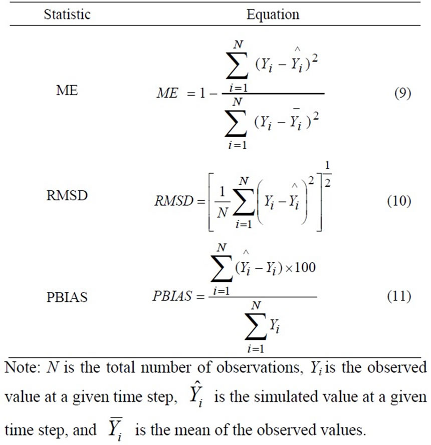
Table 5. Model performance statistics.
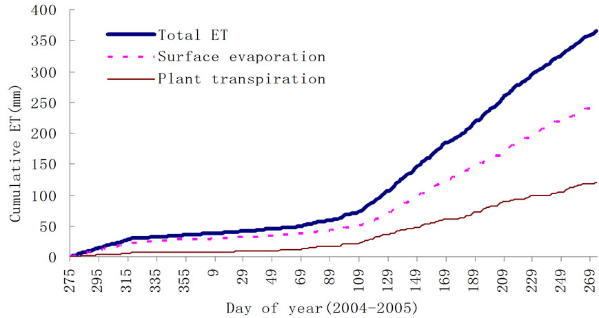
Figure 5. Simulated cumulative evapotranspiration, plant transpiration and surface evaporation for 2005 hydrologic year.
from their mean ET rate for March to September of 1998 was 1.83mm/day.
Thus, it can be concluded that SHAW model is applicable for estimating evapotranspiration from the coniferous forest in alpine region of the eastern Tibetan Plateau. As long as appropriate parameters are determined, SHAW can estimate ET quite well. This provides a good base for further application of SVAT models to the dark coniferous forest in the eastern Tibetan Plateau.
3. Results
Daily evapotranspiration was simulated for October 2004 to September 2005 after we assessed the model performance. Then, based on the simulated values, daily and seasonal variations of the key hydrologic processes of the dark coniferous forest in the eastern Tibetan Plateau were analyzed. Then the main factors influencing evapotranspiration were listed and discussed.
3.1. Evapotranspiration Variation
Evapotranspiration in SHAW includes transpiration from three plant types, and evaporation from canopy interception of precipitation, surface litter interception, and the soil surface. Figure 5 gives the cumulative evapotranspiration, plant transpiration and surface evaporation throughout the simulated period. Here, surface evaporation contains soil evaporation and evaporation intercepted precipitation from canopy and litter. Plant transpiration cumulates slow as shown in Figure 5, especially in cold season when there is scarcely any transpiration, while surface evaporation had a relative quick rise in particular for day 120 to 150 (May 2005). As a result, for the whole hydrologic year, the total ET was 366mm, of which plant transpiration accounted for 120mm, and surface evaporation for 246mm. In this study, peak ET rate occurred at day 207 (July 26), the typical bright day, at a rate of approximately 3.7mm/day (shown in Figure 6). As for sea-
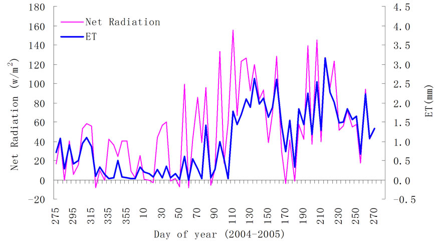
Figure 6. Daily variation of evapotranspiration and net radiation of 2004-2005.
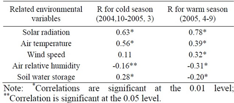
Table 6. Pearson’s correlation coefficient (R) between related environmental variables and evapotranspiration for cold and warm seasons.
sonal variation, evapotranspiration dynamics had two peak periods, one was in May, and the other was in July. The main reason is that solar radiation is intensive in May and July (this can be noticed from Figure 6).
Daily ET generally mimicked the variation in net radiation as shown in Figure 6. This supports the viewpoint brought forward by Isard and Belding [30] that with high soil moisture (a common situation in the alpine zone), evapotranspiration has been shown to linearly correlate with net radiation. This phenomenon results from at least two facts: 1) Soil water pool is sufficient to supply soil evaporation and plants transpiration. 2) Net radiation is the main driving force for evapotranspiration. Figure 7 shows the dynamics of soil water stored in the 100cm soil layer from June to October of 2005 year. It is noticed that soil water content generally maintained at a high level around 41% in this site. This means that soil water may not be the limiting factor to evapotranspiration, and the atmosphere conditions are the main factors affect ET. As for net radiation, we noticed that the Bowen ratio was low and the daily mean value was 0.15. This indicates that a high fraction of solar radiation is converted to latent heat. The comparatively low Bowen ratio also has been found in other humid high altitude zone. For instance, Tappeiner and Cernusca [31] noted that the Bowen ratio of closed vegetation was commonly below 0.5, and rarely above 1 in the central Caucasus.
In addition, we find that the link between ET and net radiation is different in cold season and warm season from Figure 6; in warm season the link is tighter than in cold season. So, in order to further illuminate which are the main factors of daily evapotranspiration in the humid faber fir forest, we analyzed the relationships between
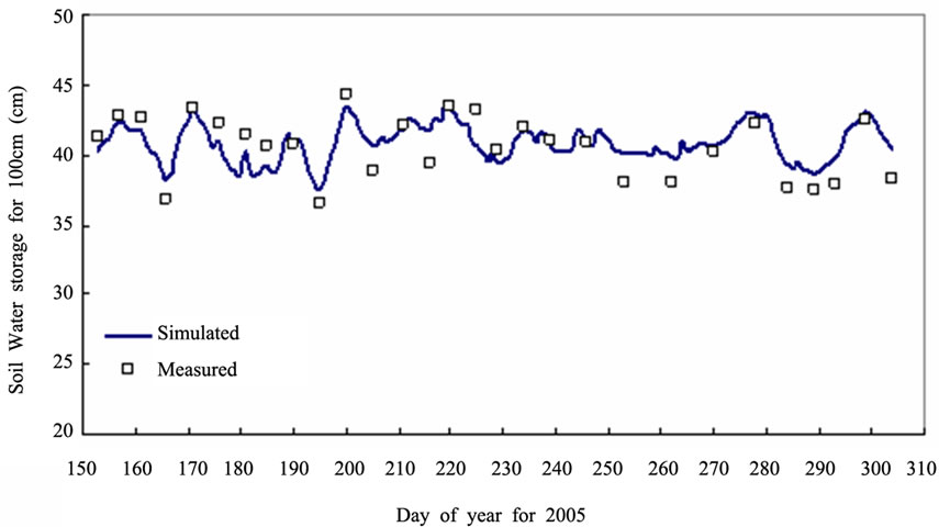
Figure 7. Dynamics of Soil water storage of 100cm soil layer form Jun. to Oct. of 2005 year.
In addition, we find that the link between ET and net radiation is different in cold season and warm season from Figure 6; in warm season the link is tighter than in cold season. So, in order to further illuminate which are the main factors of daily evapotranspiration in the humid faber fir forest, we analyzed the relationships between the environmental variables and ET using Pearson’s correlation coefficient (R). Taking into account there may be different impact intensity in different seasons, we separated 2005 hydrologic year into two seasons: the period of October 2004 to March 2005 regarded as cold season, and April to September 2005 for warm season. These environmental variables includes solar radiation, air temperature, wind speed, air relative humidity and soil water storage of 100cm soil layer considered to affect ET. Here, daily mean values of these environmental variables were used. Table 6 gives R values for the two seasons between the environmental variables and evapotranspiration. It is noticed that solar radiation is the superior factor relating to ET. This further confirms the fact that net radiation is the main driving force for evapotranspiration mentioned above. Air temperature is the second factor for evapotranspiration, but, the relative extent of importance is different in cold and warm season. In cold season, air temperature becomes important relatively compared to itself in warm season. From Figure 6, we also can find the evidence that the solar radiation has been shown a comparatively weak correlation with ET in cold season. The correlation between wind speed and ET is weak, especially in cold season. It should be mentioned that daily wind speed variation is small in the forest and wind speed usually maintains a low annual daily mean value of around 0.6m/s, and about 0.4m/s in cold season. Hence, wind speed should not be a major factor of concern for ET in the forest. There is feeble negative correlation between air relative humidity and ET. Daily air relative humidity variation is small in the forest and air relative humidity generally maintains around 90%. Interestingly, the correlation between soil water storage and ET presents opposite status in cold and warm season. From Figure 5, it is noticed that most ET is comprised of surface evaporation in cold season, whereas surface evaporation mainly comes from soil due to the less precipitation and less intercepted by canopy and litter in cold season. Hence, ET depends on supply of soil water to some extent in cold season. However, in warm seasonthe weak negative correlation between soil water storage and ET indicates that soil water is not the limiting factor to ET. In general, there is no distinct correlation between soil water and ET.
Taking into consideration that the ET in cold season accounts for only about 20% of the total ET for 2005 hydrologic year, we ranked the relevant environmental factors impacting ET according to Pearson’s correlation coefficient for warm season. As a result, solar radiation is the most important impact factor on ET, air temperature is the secondary, wind speed and air relative humidity are minor, and soil water storage is the least important of all related factors.
3.2. Water Balance
For 2005 hydrologic year, the total simulated ET was 366mm, of which plant transpiration was 120mm, and only accounted for 33%. This is relative with the physiological characteristics of the faber fir forest. The total precipitation of 2005 hydrologic year was 2042mm, of which ET accounted for 18%. In contrast, 70% of annual precipitation leaves temperate zone low altitude sites in the form of water vapor, of which roughly two thirds passes through plants [32]. The ET and the ET/P ratio from different forest ecosystems are given in Table 7. The ET and ET/P ratio for this site are lower than the relative dryer faber fir ecosystem at the other site of the eastern Tibetan Plateau, which are 520-564mm and 30-40% respectively. The low ET from the faber fir forest may be attributed to high-elevation, high atmospheric humidity and low annual temperature. In other words, the water discharge at this site and likely many other humid high-altitude sites is largely liquid, driven by runoff and seepage rather than evaporative fluxes. This is an important point for ecosystem stability, because it underlines the significance of mechanical properties of plants, for protecting alpine slopes from surface erosion.
4. Discussion
The structure of the faber fir forest ecosystem in eastern Tibetan Plateau is complicated. The vegetation is comprised of arbor, shrub and herbage, and soil is covered by residue. It is difficult to simulate evapotranspiration from the complex forest ecosystem such as evaporation from surface of soil and canopy and transpiration from vegetation synchronously using a single layer model or a double layer model. For example, Penman-Monteith equation as a single layer model regards vegetation canopy and soil as one layer, takes the characteristics of atmosphere and plant physiology into account, can explain evapotranspiration processes and illuminate the factors influencing evapotranspiration. Based on Penman-Monteith equation many model for simulating evapotranspiration were developed; however, Penman-Monteith equation is only applicable in the condition that the ration were developed; however, Penman-Monteith equation is only applicable in the condition that the ground surface is whole covered by low and short vegetation [39]. Shuttleworth-Wallce equation [40] as one representative model of the double layer models separates an ecosystem into soil layer and vegetation layer. But it is suitable to simulate evapotranspiration from sparse vegetation only and when the vegetation is not comprised by a single type it is incapable to describe the water flux from every element [41].
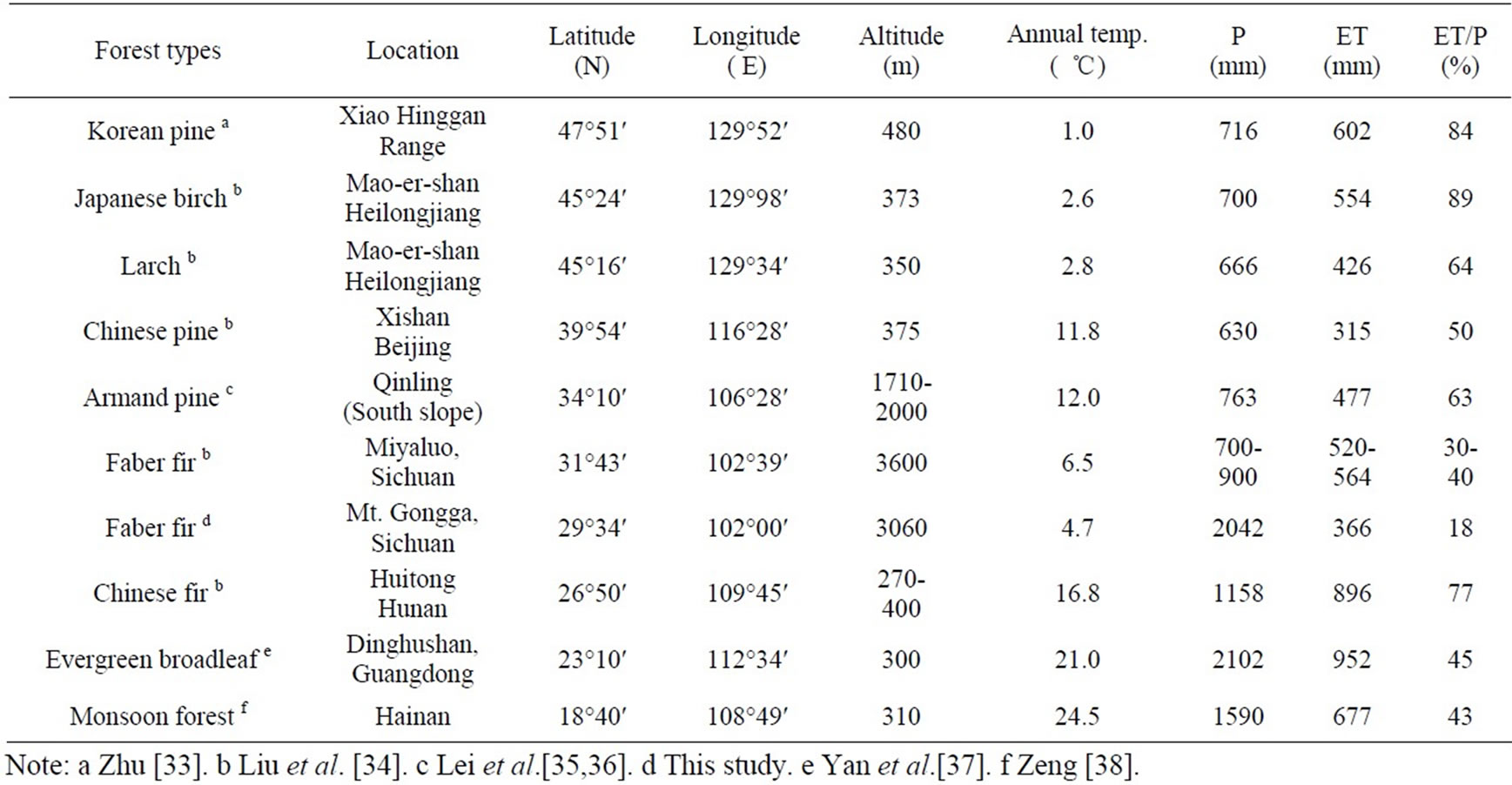
Table 7. Comparison of ET and ET/P ratio from different types of forest ecosystems.
Note: a Zhu [33]. b Liu et al. [34]. c Lei et al.[35,36]. d This study. e Yan et al.[37]. f Zeng [38].
ground surface is whole covered by low and short vegetation [39]. Shuttleworth-Wallce equation [40] as one representative model of the double layer models separates an ecosystem into soil layer and vegetation layer. But it is suitable to simulate evapotranspiration from sparse vegetation only and when the vegetation is not comprised by a single type it is incapable to describe the water flux from every element [41].
As a detailed multilayer model, the SHAW model can simulate evapotranspiration from at most 10 layers canopy with different height and physiological trait and residue layer. In this paper, the canopy of the faber fir forest ecosystem was divided into 3 layers and the residue was took as a special layer, then the total evapotranspiration from the ecosystem was evaluated by comparing with the calculated result of Bowen ratio method using measured data. Overall, the SHAW model performed well. This provides a good base for further application of SVAT models to the forest ecosystem in the eastern Tibetan Plateau.
By analysis of simulated ET using the SHAW model after calibrated and validated, some conclusions are attained:
1) Daily plant transpiration is low, and daily ET mainly comes from surface evaporation including canopy, litter and soil evaporation.
2) Daily ET has been shown to linearly correlate with net radiation due to the high soil moisture; the link between ET and net radiation is particularly during the warm season. Daily mean Bowen ratio value was 0.15, implying that a high fraction of solar radiation is converted to latent heat.
3) Solar radiation is the most important impact factor on ET, air temperature is the secondary, wind speed and air relative humidity is minor, and soil water storage is the least important of all related factors.
4) Annual ET of the faber fir forest ecosystem in eastern Tibetan Plateau is 366mm, accounting for 18% of the precipitation, this is lower compared with the other forest ecosystems owing to high-elevation, high atmospheric humidity and low annual temperature. The water discharge at this site and likely many other humid high- -altitude sites is largely liquid, driven by runoff and seepage rather than evaporative fluxes. This point is important for water resource protection and soil conservation.
5. Acknowledgements
This research was supported by the National Basic Research Program of China (No. 2005CB422005) and the National Basic S&T Project of China (No. 2006FY 110200). We thank Dr. G.W. Cheng and Gongga Mountain alpine ecosystem observation and experiment Station of Chinese Academy of Sciences for providing the meteorological and vegetation data. We would like to express our gratitude to X. D. Wang and B. R. Chen for their cooperation and assistance in collecting data. We are grateful to the reviewers for their valuable comments and suggestions on this paper.
REFERENCES
- J. M. Bosch and J. D. Hewlett, “A review of catchment experiments to determine the effect of vegetation changes on water yield and evapotranspiration,” Journal of Hydrology, Vol. 55, pp. 3–23, 1982.
- G. W. Cheng, X. H. Zhong, and Y. C. He, “The paradox and newly acquaint with the research in forest hydrology,” (In Chinese) Nature Explore, Vol. 15, pp. 81–85, 1996.
- G. W. Cheng, X. X. Yu, and Y. T. Zhao, “The hydrological cycle and its mathematical models of forest ecosystem in mountains,” (In Chinese) Science Press, Beijing, 2004.
- M. Bollasina and S. Benedict, “The role of the Himalayas and the Tibetan Plateau within the Asian monsoon system,” Bulletin of the American Meteorological Society, Vol. 85, pp. l001–1004, 2004.
- P. J. Sellers, D. A. Randall, G. J. Collatz, J. A. Berry, C. B. Field, D. A. Dazlich, C. Zhang, G. D. Collelo, and L. Bounoua, “A revised land surface parameterization (SiB2) for atmospheric GCMs, Part I: Model formulation,” Journal of Climate, Vol. 9, pp. 676–705, 1996.
- G. N. Flerchinger, C. I. Hanson, and J. R. Wight, “Modeling of evapotranspiration and surface energy budgets across a watershed,” Water Resources Research, Vol. 32, pp. 2539–2548, 1996.
- S. Sitch, B. Smith, I. C. Prentice, A. Arneth, A. Bondeau, W. Cramer, J. O. Kaplan, S. Levis, W. Lucht, M. T. Sykes, K. Thonicke, and S. Venevsky, “Evaluation of ecosystem dynamics, plant geography and terrestrial carbon cycling in the LPJ dynamic global vegetation model,” Global Change Biology, Vol. 9, pp. 161–185, 2003.
- G. N. Flerchinger and K. E. Saxton, “Simultaneous heat and water model of freezing snow-residue-oil systemⅠtheory and development,” Transactions of American Society of Agricultural Engineers, Vol. 32, pp 565–571, 1989.
- G. N. Flerchinger and K. E. Saxton, “Simultaneous heat and water model of freezing snow-residue-soil system Ⅱ field verification,” Transactions of American Society of Agricultural Engineers, Vol. 32, pp. 573–578, 1989.
- G. N. Flerchinger and F. B. Pierson, “Modeling plant canopy effects on variability of soil temperature and water: Model calibration and validation,” Journal of Arid Environment, Vol. 35, pp. 641–653, 1997.
- G. N. Flerchinger, K. R. Cooley, and Y. Deng, “Impacts of spatially and temporally varying snowmelt on subsurface flow in a mountainous watershed snowmelt simulation,” Hydrologic Sciences Journal, Vol. 39, pp. 507–520, 1994.
- G. N. Flerchinger, J. M. Baker, and E J. Spaans, “A test of the radiative energy balance of the SHAW model for snow cover,” Hydrological Processes, Vol. 10, pp. 1359–1367, 1996.
- H. N. Hayhoe, “Field testing of simulated soil freezing and thawing by the SHAW model,” Canadian Agriculttural Engineering, Vol. 36, pp. 279–285, 1994.
- G. M. Preston, “An analysis of SHAW model water budget estimations for municipal solid waste landfill covers planted with poplar tree systems in southern Ontario,” Master of Science Thesis. University of Guelph, Canada, 2002.
- T. E. Link, G. N. Flerchinger, M. H. Unsworth, and D. Marks, “Simulation of water and energy fluxes in an old growth seasonal temperate rainforest using the Simultaneous Heat and Water (SHAW) Model,” Journal of Hydrom-eteorology, Vol. 5, pp. 443–457, 2004.
- I. S. Bowen, “The ratio of heat losses by conduction and evaporation from any surface,” Physics Review, Vol. 27, pp. 779–789, 1926.
- C. B. Tanner, “Energy balance approach to evapotranspiration from crops,” Soil Science Society of America Processes, Vol. 24, pp. 1–9, 1960.
- N. J. Rosenberg, B. L. Blad, and S. B. Verma, “Microclimate: the biological environment,” John Wiley, New York, pp. 495, 1983.
- S. O. Ortega-Farias, R. H. Cuenca, and M. Ek, “Daytime variation of sensible heat flux estimated by the bulk aerodyne--mic method over a grass canopy,” Agricultural and Forest Meteorology, Vol. 81, pp. 131–143, 1996.
- H. E. Unland, P. R. Houser, W. J. Shuttleworth, and Z. L. Yang, “Surface flux measurement and modelling at a semi-arid Sonoran Desert site,” Agricultural and Forest Meteorology, Vol. 82, pp. 119–153, 1996.
- P. J. Perez, F. Castellvi, and M. Ibanez, “Assessment of reliability of Bowen ration methods for partitioning fluxes,” Agricultural and Forest Meteorology, Vol. 97, pp. 141–150, 1999.
- G. N. Flerchinger and F. B. Pierson, “Modeling plant canopy effects on variability of soil temperature and water,” Agricultural and Forest Meteorology, Vol. 56, pp. 227–246, 1991.
- G. S. Campbell, “Soil Physics with BASIC: Transport models for soil-plant systems,” Elsevier, Amsterdam, 1985.
- G. N. Flerchinger, “The simultaneous heat and water (SHAW) model: Technical documentation,” Northwest Watershed Research Center USDA Agricultural Research Service, Boise, Idaho, 2000.
- G. N. Flerchinger, “the simultaneous heat and water (SHAW) model: User’s manual,” 2003. [Available online at ftp://ftp.nwrc.ars.usda.gov/public/Shawmodel/ ]
- G. S. Campbell, “An introduction to environmental biophysics,” Springer-Verlag, New York, 1977.
- J. Luo, G. W. Cheng, M. Q. Song, and W. Li, “The characteristics of litter fall of Abies Fabri forests on the Gongga Mountain,” (In Chinese with English abstract) Acta Phytoecologica Sinica Vol. 27, pp. 59–65, 2003.
- Q. T. He, “China forest meteorology,” (In Chinese) China Forestry Publishing House. Beijing, 2001.
- G. W. Cheng, X. X. Yu, Y. T. Zhao, Y. M. Zhou, and J. Luo, “Evapotranspiration simulation of subalpine forest area in Gongga Mountain,” (In Chinese with English abstract) Journal of Beijing Forestry University. Vol. 25, pp. 23–27, 2003.
- S. A. Isard, M. J. Belding, “Evapotranspiration from the alpine tundra of Colorado, U.S.A.” Resistance and resilience of tundra plant communities to disturbance by winter seismic vehicles. Arctic and Alpine Research, Vol. 21, pp. 71–82, 1989.
- U. Tappeiner and A. Cernusca, “Microclimate and fluxes of water vapour, sensible heat and carbon dioxide in structurally differing subalpine plant communities in the central Caucasus,” Plant cell Environment, Vol. 19, pp. 403–417, 1996.
- Ch. Korner, “Alpine plant life, functional plant ecology of high mountain ecosystems,” Springer, Berlin Heidelberg New York, pp. 121–126, 2001.
- J. W. Zhu, “Water balance of Korean pine stand and its cutting blank,” (in Chinese) Acta Ecologica Sinica, Vol. 34, pp. 12–21, 1982.
- S. Liu, P. Sun, and J. Wang, “Hydrological functions of forest vegetation in upper reaches of Yangtze River,” (In Chinese with English abstract) Journal of Natural Resources, Vol. 16, pp. 451–456, 2001.
- R. Lei, L. Shang, and Z. Tang, “The influence of human activities on hydrological functions of a Quercus aliena forest,” (in Chinese) In Zhou X (ed.) “Studies on forest ecosystems,” Northeast Forestry University Press, Harbin, pp .235–244, 1994.
- R. Lei, Y. Zhang, and K. Dang, “A study on hydrological effects of forest in the Qinling Mountains Forest Region,” (in Chinese) In Zhou X (ed.) “Studies on Forest Ecosystems”, Northeast Forestry University Press, Harbin, pp. 223–234. 1994.
- J. Yan, G. Zhou, and Z. Huang, “Evapotranspiration of the monsoon evergreen broad-leaf forest in Dinghushan,” (in Chinese) Scientia Silvae Sinica, Vol. 37, pp. 37–45, 2001.
- Q. Zeng, “Monsoon forest water cycle of Jianfeng mountain of Hainan province,” (in Chinese) In Zhou X (ed.) “Studies on forest ecosystems,” Northeast Forestry University Press, Harbin, pp. 413–429, 1994.
- C. M. Liu and H. X. Wang, “Soil-crops-atmosphere interface water processes and water saving control,” (in Chinese) Science Press, Beijing, 1999.
- W. J. Shuttleworth and J. S. Wallance, “Evaporation from sparse crops-an energy combination theory,” Quarterly Journal of the Royal Meteorological Society, Vol. 111, pp. 839–855, 1985.
- J. M. Norman, W. P. Kusts, and K. S. Humes, “Source approach for estimating soil and vegetation energy fluxes in observations of directional radiometric surface temperature,” Agricultural and Forest Meteorology, Vol. 77, pp. 263–293, 1995.