Received 30 April 2015; accepted 27 June 2015; published 30 June 2015

ABSTRACT

This part II-C of our work completes the factorizational theory of asymptotic expansions in the real domain. Here we present two algorithms for constructing canonical factorizations of a disconjugate operator starting from a basis of its kernel which forms a Chebyshev asymptotic scale at an endpoint. These algorithms arise quite naturally in our asymptotic context and prove very simple in special cases and/or for scales with a small numbers of terms. All the results in the three Parts of this work are well illustrated by a class of asymptotic scales featuring interesting properties. Examples and counterexamples complete the exposition.

Keywords:

Asymptotic Expansions, Canonical Factorizations of Disconjugate Operators, Algorithms for Canonical Factorizations, Chebyshev Asymptotic Scales

12. A Third Heuristic Approach to Factorizational Theory

We continue the numbering of sections used in the preceding two parts of this work: Part II-A [1] , and Part II-B [2] . In the survey ([3] , §3) we highlighted two heuristic approaches leading to two Conjectures whose proofs appear in [1] [2] in a completed form. We are going to illustrate another way to arrive at the second Conjecture, ([3] , p. 12), by the elementary use of L’Hospital’s rule. In our endeavor to find sufficient and/or necessary conditions for the validity of an asymptotic expansion

(12.1)

where the asymptotic scale

(12.2)

is subject to certain Wronskian restrictions, let us try to find out expressions for the coefficients alternative to the elementary (and rarely useful) iterative formulas:

(12.3)

where the existence (as finite numbers) of the involved limits characterize the coefficients whenever the’s do not vanish on a deleted neighborhood of. Let us now heuristically try to evaluate the first few limits above by L’Hospital’s rule:

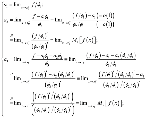(12.4)

where by (2.35) M₁, M₂ are the operators defined in (3.3), apart from the signs. By iteration we may conjecture that this heuristic procedure leads to the formulas

(12.5)

provided the involved limits exist in; and these formulas are true, apart from the signs, whenever the remainder in (12.1) is identically zero ([1] , Prop. 3.1). Such kind of manipulations may seem artificial and awkward from an elementary viewpoint and it is by no means obvious that iteration of the procedure yields (12.5).

・ In §13 we show that different organizations of the above calculations give rise to two algorithms for constructing canonical factorizations starting from a given asymptotic scale; the procedures seem quite natural in the context of formal differentiation of an asymptotic expansion and shed a light of “easiness”, so to say, on the formulas of asymptotic differentiability obtained so far and seemingly complicated in themselves.

・ In $14 an example illustrating the two algorithms is given.

・ In §15 a useful class of scales is studied highlighting some pecularities concerning various types of formal differentiabilty and here the idea underlying the two algorithms plays a role even if manipulated differently.

・ The last §16 contains additional remarks on the algorithms.

13. Constructive Algorithms for Canonical Factorizations

The original procedure used by Trench [4] to construct a C.F. of type (I) for a disconjugate operator is not an intuitive one but, besides its historical value, it shows the existence of such a factorization separately at each endpoint of the interval of disconjugacy; this fact in turn shows the existence of a basis of ker forming an asymptotic scale at each fixed endpoint. But in the theory we have been developing the starting point is different, namely it is such an asymptotic scale. Here we exhibit two easy algorithms to construct both types of C.F.’s starting from an explicit basis of ker forming an asymptotic scale at one endpoint. The so-obtained factorizations will be proved to coincide with those obtainable by Pólya’s procedure when applied either to the asymptotic scale or to the inverted n-tuple so providing alternative constructive ways to such factorizations. Each step in the algorithms has an asymptotic meaning and the algorithm for a C.F. of type (II) is particularly meaningful as it highlights how the operators naturally arise from an asymptotic expansion with an identically-zero remainder when one attempts to find out independent expressions for each of its coefficients. Both algorithms may sometimes be quicker to apply than Pólya’s procedure, especially for small values of n, avoiding the explicit use of Wronskians.

Let us consider a generic element of the type

(13.1)

which we interpret as an asymptotic expansion at (with a zero remainder). We shall first present the algorithm for a C.F. of type (II) as it is more simple to describe.

Theorem 13.1 (The algorithm for a special C.F. of type (II)). Let satisfy conditions (2.23), (2.24), (2.25) in Part II-A with all the Wronskians strictly positive; then the following algorithm yields the special glob-

al C.F. of of type (II) at x₀ in (2.39) [1] , together with asymptotic expansions which, after di-

viding by the first meaningful term on the right, concide with the expansions obtained by applying to (13.1) the operators defined in (3.3) [1] . The formulas for the coefficients in (3.18) [1] , with, are reobtained.

(A) Verbal description of the algorithm.

1^st step. Divide both sides of (13.1) by the first term on the right, which is the term with the largest growth- order at, and then take derivatives so obtaining

(13.2)

Suppressing the derivative the left-hand side in (13.2) is the operator M₀u.

2^nd step. Divide both sides of (13.2) by the first term on the right and take derivatives so obtaining

(13.3)

Suppressing the outermost derivative the left-hand side in (13.3) is the operator M₁u.

3^rd step. Repeat the procedure on (13.3) dividing by the first term on the right and then taking derivatives so getting

(13.4)

Iterating the procedure each of the obtained relation is an identity on and is an asymptotic expansion at x₀, hence at each step we are dividing by the term on the right with the largest growth-order at x₀. Notice that at each step the asymptotic expansion loses its first meaningful term and this is the same phenomenon occurring in differentiation of Taylor’s formula. After n steps we arrive at an identity

(13.5)

where the’s coincide with those in (2.35).

(B) Schematic description of the algorithm.

Step “1”:

Step “2”:

Step “3”:

Step “4”:

and so on, where the symbol “d & d” stands for the two operations “divide” both sides by the underbraced term on the right and then “differentiate” both sides (the equation in each step being the result of the preceding step).

Theorem 13.2 (The algorithm for the C.F. of type (I)). Let satisfy conditions (2.23), (2.24), (2.25) in Part II-A; then the following algorithm yields “the” global C.F. of of type (I) at x₀ and asymptotic expansions which, after dividing by the last meaningful term on the right, coincide (apart from the signs of the coefficients) with the expansions obtained by applying to (13.1) the operators defined in (3.1) [1] .

(A) Verbal description of the algorithm.

1^st step. Divide both sides of (13.1) by the last term on the right, which is the term with the smallest growth- order at, and then take derivatives so obtaining

(13.6)

2^nd step. Divide both sides of (13.6) by the last term on the right and then take derivatives so obtaining

(13.7)

3^rd step. Repeat the procedure on (13.7) dividing by the last term on the right and then taking derivatives so getting

(13.8)

Iterating the procedure each of the obtained relation is an identity on and is an asymptotic expansion at x₀, hence at each step we are dividing by the term on the right with the smallest growth-order at x₀. Also notice that at each step the asymptotic expansion loses its last meaningful term and this is a phenomenon different from that occurring in differentiation of Taylor’s formula (see the foregoing proposition). After n steps we arrive at an identity

(13.9)

where the’s coincide, signs apart, with those in (2.43).

(B) Schematic description of the algorithm.

Step “1”:

Step “2”:

Step “3”:

Step “4”:

and so on with the symbol “d & d” reminding of the two operations “divide” both sides by the underbraced term on the right and then “differentiate” both sides (the equation in each step being the result of the preceding step).

Remarks. 1) In order to obtain any C.F. by the above procedures one may simply choose.

2) If some operator is known to be disconjugate on a left neighborhood of, and if

(13.10)

then the algorithm in Theorem 13.2 yields the C.F. of type (I) at x₀, valid on the whole given interval whereas the algorithm in Theorem 13.1 yields a C.F. of type (II) at x₀ valid on some left neighborhood of x₀, the largest of them being characterized by the nonvanishingness of all the Wronskians, which does not automatically follow from the nonvanishingness of,. These facts follow from Proposition 2.2-(I) in Part II-A. We remind the reader that if is any basis of ker then there is a simple algebraic procedure to construct another basis forming an asymptotic scale at, Levin ([5] , Lemma 2.1, p. 58).

3) In practical applications of the algorithms there is a fatal pitfall to avoid, namely the temptation at each step of suppressing brackets, cancelling possible opposite terms and rearranging in an aestetically-nicer asymptotic scale. This in general gives rise to a factorization of an operator quite different from. Hence it is essential that all the terms coming from a single term in the preceding step be kept grouped together as a single term to the end of the procedure: see examples in §14.

4) The algorithms are of course applicable to obtain C.F.’s at a left endpoint valid on each neighborhood whereon the Wronskians never vanish.

Proof of Theorem 13.1, that of Theorem 13.2 being exactly the same after replacing by. We first prove that the’s in (13.5) coincide with those in (2.35) [1] , and this does not seem an obvious fact though it is made explicit in the algorithm that the first three coefficients q₀, q₁, q₂ coincide with Pólya’s coefficients in (2.35) [1] . Now, known, our algorithm constructs, for, by the following rule:

(13.11)

hence it is enough to show that Pólya’s expression for is obtained by the same rule. We present two different proofs, the first being based on the equivalent representations (2.35) and (2.37) in [1] . We have:

(13.12)

It is also clear that the various identities obtained are nothing but those obtained by applying to (13.1) the operators defined in (3.3) which, by (3.12), differ from by a factor which is a non-vanishing function. We wish to present a second proof based on a nontrivial identity involving Wronskians of Wronskians, Karlin ([6] , p. 60), which we report here in the version needed in our proof:

(13.13)

Comparing the expressions in (2.37) [1] , and those given by our algorithm we see that the two procedures coincide if the following identity holds true:

(13.14)

We shall show the validity of this identity even if the outermost derivatives are suppressed. Using the elementary formula we have:

(13.15)

by (13.13) with replaced by

We have also proved that at the k-th step the linear combination on the right, before dividing for the next step, coincides with the expression

which, by (3.8) in Part II-A, is an asymptotic expansion at. The proof is over.

14. Examples Illustrating the Two Algorithms

Consider the fourth-order operator L of type (2.1)_1,2, [1] , such that

(14.1)

acting on or even on. Starting from the asymptotic scale

(14.2)

the algorithm in Theorem 13.2 yields in sequence:

Hence

(14.3)

and this is “the” global C.F. of L of type (I) at. On the other hand the algorithm in Theorem 13.1 yields in sequence:

(The underbraced terms on the right are those by which one must divide and then differentiate.) Hence:

(14.4)

where

(14.5)

Hence (14.4) is a C.F. of L of type (II) at valid on the largest neighborhood of whereon

which is easily seen to be the interval. In conclusion: changing the signs of the’s, if necessary, we get a Pólya-Mammana factorization of L on which is a C.F. of type (II) at. The standard non- factorized form of L is

(14.6)

In the various steps of the above procedures one must carefully avoid the temptation of rearranging the terms in the right-hand side in (supposedly) nicer asymptotic scales. For instance the first procedure involves quite simple terms and only at the last-but-one step we may split the remaining term on the right by writing

and taking as the term with the smallest growth-order. The procedure then yields

This gives a fifth-order operator

(14.7)

distinct from the given fourth-order operator. On the contrary the second procedure offers a great number of temptations! For instance if one rewrites the result of the first step as

(14.8)

and then goes on applying the second algorithm to (14.8) as if the right-hand side would be an asymptotic expansion with three meaningful terms, one gets:

(14.9)

the only difference between the two expressions on the right being the term-grouping. From the upper relation in (14.9), considered as an asymptotic expansion at with two meaningful terms, one gets:

and then

(14.10)

whose left-hand side is a fourth-order operator distinct from our operator. If, instead, one starts from the lower relation in (14.9), considered as an expansion at with three meaningful terms, one gets:

and so forth in an endless process leading nowhere!!

15. A Special Class of Chebyshev Asymptotic Scales

15.1. Preliminaries

We specialize the results of our theory for the special class of Chebyshev asymptotic scales

(15.1)

where

(15.2)

Our assumptions will be:

(15.3)

This class has been cursorily presented in ([3] , §7) but will receive here a detailed treatment highlighting how the ideas of our algorithms may lead to discover new facts about formal differentiability. The class contains meaningful and frequently-used scales exhibited at the end of the section.

To apply our theory we observe that by a proper device it can be given an elementary proof of the formula (which is anyway a classical result):

(15.4)

where denotes the Vandermonde determinant of the n distinct numbers; hence our assumptions imply the non-vanishingness of all the Wronskians involved in our theory and the scale (15.1) turns out to be a Chebyshev asymptotic scale on. Putting, formulas in ([1] , Prop. 2.4) give the C.F.’s

of the differential operator associated to our scale apart from the signs and neglecting all the

various constant factors appearing in the expressions of the Wronskians. Hence, apart from immaterial constant factors, the functions, may be defined by

(15.5)

(15.6)

Proposition 15.1 (C.F.’s for the asymptotic scale (15.1)). Let and the n-tuple satisfy conditions (15.2), (15.3) and let be the differential operator associated to the scale (15.1). Then, apart from the signs of the coefficients:

(I) The “unique” C.F. of type (I) at is

(15.7)

and we denote by, the differential operator of order k corresponding to the defined in ([1] ; formula (3.1)).

(II) A special C.F. of type (II) at is

(15.8)

and we denote by, the differential operator of order k corresponding to the defined in ([1] , formula (3.3)).

The above factorizations may quite simply be obtained via our algorithms as well; for instance starting from

(15.9)

the procedure of the second algorithm yields in sequence:

and so on (15.7) follows. If, as a first step, both sides of (15.9) are divided by then the procedure of the first algorithm yields (15.8). But in this specific case, beside the fact that the algorithms yield C.F.’s of the two types, it is almost a matter of instinct to apply standard derivatives to both sides in (15.9), then dividing by and iterating the procedure so getting in sequence:

(15.10)

and no matter how many times we iterate the procedure the right sides is a non-identically zero expression except for special sequences of the exponents such as or. Hence as regards factorizations the last procedure is unrelated to the operator; but if in the asymptotic expansion (15.9) we add a non-zero remainder then, referring to (15.10), formally-differentiated expansions such as

(15.11)

seem natural contingencies quite likely to be encountered. We shall show that the two main sets af expansions characterized in our theory actually are equivalent to expansions involving iterates of the simple operator and that relations like those in (15.11) hold true under a strong assumption on the given function: in fact this is the case in Proposition 15.3 but not in Proposition 15.2 below. Hence we define the following differential operators dependent on but not on:

(15.12)

noticing the identities

(15.13)

The second identity in (15.13) is the main operational property of. In passing notice that

(15.14)

15.2. Weak and Strong Formal Differentiability

We report only on “complete” asymptotic expansions; for “incomplete” expansions it might be complicated to list all the circumstances concerning estimates of the remainders: see Theorem 9.2-(II) in Part II-B.

Proposition 15.2. (Characterizations of “weak” formal differentiability for the scale (15.1)).

(I) Referring to Theorem 4.5 in [1] we have the equivalence of the following four properties:

1) The set of asymptotic expansions as for suitable constants:

(15.15)

where denotes the linear combination.

2) The set of asymptotic expansions as for suitable constants:

(15.16)

3) The improper integral

(15.17)

4) For suitable constants the following representation holds true on:

(15.18)

(II) The linear combinations in the two types of differentiated expansions are explicitly given by

(15.19)

wherein the second sum actually denotes the expression of truncated at the order. Notice that the differentiated expansions in (15.15) and (15.16) share the phenomenon that the last term in each expansion is lost in the successive expansion but this happens for different reasons. In (15.15) it is each operator which annihilates the last term whereas in (15.16) no term in the expression of is annihilated for a generic sequence but the last term must be suppressed due to the estimate of the remainder and this is the import of the Proposition.

Proposition 15.3. (Characterizations of “strong” formal differentiability for the scale (15.1)).

(I) Referring to Theorem 5.1 in [1] we have the equivalence of the following four properties:

1) The set of asymptotic expansions as for suitable constants:

(15.20)

2) The set of asymptotic expansions as for suitable constants:

(15.21)

3) The improper integral

(15.22)

4) For suitable constants the following representation holds true on:

(15.23)

(II) The linear combinations in the two types of differentiated expansions are explicitly given by

(15.24)

wherein the second sum, generally speaking, contains all the terms in the expression of. Hence in this case the differentiated expansions in (15.20) are such that the first term in each expansion is lost in the successive expansion whereas each differentiated expansion in (15.21) contains all the meaningful terms, save exceptional cases.

Comparing (15.16) and (15.21) we see that each remainder in (15.16) has a growth-order greater than the corresponding one in (15.21) hence we may say that (15.16) and (15.21) are obtained from the first expansion in (15.15) by formal differentiation respectively in a “weak” and in a “strong” sense: see Remark and Open Problem at the end of §8 in [2] . From an algebraic viewpoint the estimates of the remainders in (15.21) seem to be the most natural possible but actualy they hold true only under a strong assumption. To visualize, notice that expansions in (15.21) correspond to the formal procedure in (15.11), starting from (15.9) with a remainder inserted, whereas expansions in (15.16) correspond to the following formal procedure

(15.25)

Propositions 15.2 and 15.3 generalize the technical lemmas used in ([7] , Lemmas 7.3, 7.4) for real-power expansions, which is the particular choice.

Proposition 15.4. (A case of equidistant exponents). (I) If, , which is the same as, , we may write the sequence of exponents as hence it must

be. It follows from (15.7) that; so the corresponding expansions in (15.15), (15.16) are practically the same and all the remainders in the differentiated expansions in (15.16) are. Under the integral condition

(15.26)

we have the expansion for f together with the equivalent sets of differentiated expansions

(15.27)

with the coefficients made explicit in the second relation in (15.19) and wherein all the remainders have the same growth-order even if the last term is lost in the successive expansion. Only for the very particular choice we have: see (15.14). And under the stronger integral condition

(15.28)

we have the expansion for f together with the equivalent sets of differentiated expansions

(15.29)

with the coefficients made explicit in (15.24).

(II) If, which is the same as, we may write the se-

quence of exponents as hence it must be. It follows from (15.8) that and the corresponding expansions in (15.20), (15.21) are practically the same and all the remainders in the differentiated expansions in (15.21) are. Under the integral condition

(15.30)

we have the expansion for f together with the equivalent sets of differentiated expansions

(15.31)

with the coefficients, made explicit in (15.19). Here in the expansions of the exponent of each remainder decreases by two units in the successive expansion and so, due to, the growth- order of the remainder increases. And under the stronger integral condition

(15.32)

we have the expansion for f together with the equivalent sets of differentiated expansions

(15.33)

with the coefficients made explicit in the second relation in (15.24) and wherein the exponents appearing in the remainders decrease by one unit at each successive differentiation. Only for the very particular choice we have and in this case the first term in each expansion is lost in the successive expansion because it is annihilated by the operator: this actually is Taylor’s formula.

Writing down the first two differentiated expansions for each group may help the reader grasp the different circumstances. In the situation of Proposition 15.4-(I) and in a concise notation let us start from the expansion

(15.34)

Then the three expansions in (15.27) and (15.29) respectively run as follows:

(15.35)

(15.36)

(15.37)

For a quick check of (15.37) the reader is suggested to use the algorithm in Proposition 13.1.

Remark. The above results give a glimpse of the great variety of differentiated expansions that may be encounterd in applications. In the general case of equidistant exponents, , it happens that the coefficients in the two factorizations (15.7)-(15.8), apart from the outermost and the innermost ones, coincide with each other namely they are: in (15.7) and in (15.8); and differentiated expansions similar to those in the above proposition hold true under the appropriate assumptions.

15.3. Proofs

The proofs of Propositions 15.2, 15.3 rely on formulas linking the various involved operators.

Lemma 15.5. (I) For weak differentiability the formula linking and is

(15.38)

with suitable coefficients whose explicit expressions are not required for our aims save that.

(II) For strong differentiability the formula linking and is

(15.39)

with suitable coefficients with.

Proof. Let us prove (15.38). For we have

(15.40)

and suppose (15.38) hold true for a certain k; then for we have

which is (15.38) with k replaced by and suitable coefficients. To prove (15.39) just notice that the expression of is obtained by the expression of substituting with.

Due to the linearity of our operators it is enough to prove our claims for the case. The equivalences between (15.15) and (15.16) and between (15.20) and (15.21) are contained in the following

Lemma 15.6. With shortened notations we have:

(15.41)

(15.42)

Proof. The equivalence in (15.41) is easily checked for using (15.40) and the inverse formula

(15.43)

We assume this equivalence to hold true for a certain range and suppose that, , , then by (15.38) and the inductive assumption we get

Viceversa suppose that, ,; then the inductive assumption implies the estimates for, , and from (15.38) we get

whence

which is the sought-for estimate. The equivalence in (15.42) is similarly proved using (15.39).

15.4. Examples

We specialize the foregoing results for particular choices of which include common and useful scales at. In the following examples we write the explicit expansions involving the operators and, whenever possible, those involving the operators for the sake of comparison. To obtain an equivalent (or sometimes subordinate) set of expansions in terms of the standard derivatives we first establish a formula linking and and then apply the same kind of argument as in Lemma 15.6. It will be apparent from the examples that no general meaningful result involving standard derivatives can be obtained for this special class of expansions: for each choice of there is an interplay between algebraic and asymptotic properties. The same symbol obviously has a different meaning in each case, being the operator whose kernel is spanned by the pertinent asymptotic scale. To shorten formulas we use the notation:

(15.44)

where is termed the “kth falling (or decreasing) factorial power of”. Notice that we have defined, hence a linear combination such as simply means.

Examples for weak differentiability. (I). For any real numbers the following two properties are equivalent:

(15.45)1

(15.45)2

And under the restrictions which may be written as

(15.46)

they are equivalent to:

(15.47)

But it must be observed that, though the comparison functions appearing in each summation in (15.47) form an asymptotic scale due to the easily-checked relation

the asymptotic expansions in (15.47) are, so to say, impure in so far that neither all the terms in the explicit expressions of nor all the terms into each summation symbol are necessarily meaningful.

Under the restrictions which is the same as the reversed chain of inequalities in (15.46), the set of expansions in (15.45)₂ implies the following weaker set of expansions than in (15.47)

(15.48)

but not viceversa. The claims about (15.47) follow from the formula

(15.49)

which implies

(15.50)

under conditions (15.46). For generic values of the’s no such equivalence holds true and, if the inequalities in (15.46) are reversed, then (15.50) is replaced by the inference

(15.51)

(II). For any real numbers the following are equivalent properties:

(15.52)1

(15.52)2

(III). For and and for any real numbers the following are equivalent properties:

(15.53)1

(15.53)2

(IV). For any real numbers the following are equivalent properties:

(15.54)1

(15.54)2

(15.54)3

The equivalence between (15.54)₂ and (15.54)₃ follows from the formula

(15.55)

which implies

(15.56)

(V). For and for any real numbers the following are equivalent properties:

(15.57)1

(15.57)2

Examples for strong differentiability. (I). The following are equivalent properties:

(15.58)1

(15.58)2

Quite surprisingly we don’t have any characterization in terms of whatever the sequence; it can only be proved, using (15.49), that the set of expansions in (15.58)₂ implies (but is not implied by) the expansions

(15.59)

wherein all the terms into the summation symbol must be taken into consideration but not all the terms in the explicit expressions of are meaningful.

(II). For any real numbers the following are equivalent properties:

(15.60)1

(15.60)2

(III). For and and for any real numbers the following are equivalent properties:

(15.61)1

(15.61)2

(IV). For any real numbers the following are equivalent properties:

(15.62)1

(15.62)2

(15.62)3

The equivalence between (15.62)₂ and (15.63)₃ follows easily from (15.55).

(V). For and for any real numbers the following are equivalent properties:

(15.63)1

(15.63)2

15.5. Estimates of the Remainders in a Case of Incomplete Expansions

To illustrate Theorems 8.3-8.4 in Part II-B we exhibit the estimates of the remainders in a case of incomplete expansions for a generalized convex function with respect to the scale (15.1)-(15.3).

Proposition 15.7. Let be the operator defined in Proposition 15.1 and let a function f satisfy:

(15.64)

then the following asymptotic relations hold true as:

(15.65)

(15.66)

consistently with Corollary 8.5 in Part II-B.

Proof. Using the expressions of the’s in (15.6) it is trivial to obtain

(15.67)

with suitable non-zero constants, whence relations in (15.65) follow from Theorems 8.3-8.4. The inference “(15.65) Þ (15.66)” is proved as in Lemma 15.6. Suppose (15.65) hold true with, then by (15.39)

and by an easy induction the remaining estimates are proved.

16. Remarks on the Algorithms and Formal Differentiability

16.1. A Random Use of the Procedures in the Algorithms

What about applying the above algorithms to (13.1) with a random choice of the term to be factored out at each step? If one carefully checks that at each step one is dividing by a nowhere-vanishing function one may well obtain, after n steps, a factorization valid on a certain subinterval of the given interval but, in general for, it will not be a C.F. at one of the two endpoints of the subinterval. In the following simple example for we exhibit all the possible factorizations that can be obtained starting from a fixed asymptotic scale and applying the procedure in the algorithms. The involved identities will be used below in this section for a counterexample of theoretical interest. Let us consider acting on or even on and the tern which satisfies

and is such that all the possible Wronskians constructed with these three functions do not vanish on. All the possible variants are six and they actually lead to six different factorizations; we arrange all the procedures in the following Tables 1-3:

And here are the 6 so-obtained factorizations arranged in the same order:

(I) (16.1)

(II) (16.2)

(III) (16.3)

all valid on. Among them the first in (16.1) is a C.F. of type (I) at 0 and of type (II) at and the first in (16.3) is a C.F. of type (I) at and of type (II) at 0. None of the remaining factorizations is a C.F. at any of the endpoints.

A few remarks about the factorizations of listed in Part II-B, §11.1, formulas (11.5)-(11.7). The factorizations in (11.5), (11.6) may be obtained by the above algorithms referred to the endpoint i.e. applied to the equality; the second of these factorizations is also valid on and (signs apart) is a C.F. of type (II) at. Starting from the equality the first algorithm yields the factorization in (11.7) valid on and a C.F. of type (II) at quite different from the preceding one. The factorization in (11.7) is valid on as well but is no C.F. at each of the two endpoints.

16.2. Some Considerations on Formal Differentiability

Let be disconjugate on an open interval and let be a basis of its kernel satisfying

(16.4)

Then by Proposition 2.2 in Part II-A all the possible Wronskians, constructed with non-

coinciding’s, never vanish on some left deleted neighborhood of b and, in addition, all the Wronskians for a fixed k can be arranged in an asymptotic scale at. Now, starting from an identity (13.1), interpreted as an asymptotic expansion at with an identically-zero remainder, any random application of our algorithms leads to identities of the type

(16.5)

where the functions on the right can be arranged in an asymptotic scale at. Hence, referring to the scale in (16.4), there exist asymptotic expansions which admit of formal differentiation times according to any randomly chosen aplication of our algorithms. Our theory gives a complete description of two special types of formal differentiability, surely the most expressive ones, and the examples in §11.2, [2] , show the difficulty of similar complete descriptions for other types not linked to C.F.’s. In practical applications, if an expansion is given, one may well expect formal differentiability (if any) of any of the just pointed-out types and even with respect to a non-C.F. only. This is clarified by the following elementary but nontrivial

Examples of formal differentiability according to canonical or non-canonical factorizations. The function

(16.6)

admits of the expansion

(16.7)

with the remainder explicitly given by,. Let us now take into considerations the six factorizations in (16.1)-(16.3) and the procedures that generated them; to check if the expansion in (16.7) is formally differentiable twice according to, say, the first factorization in (15.1) one has to evaluate the first two differentiated expressions on the left in the Table 1 in §16.1, with u replaced by, and impose the conditions that they may be considered as “remainders” as. We use shortened locutions to summarize the results. For instance we say that the expansion in (16.7) has property I-A if

“inferred from the left side of Table 1”;

and it has property I-B if

“inferred from the right side of Table 1”.

Properties II-A, II-B, III-A, III-B are similarly defined looking at Table 2 and Table 3 respectively. Elementary, though tedious, calculations show that:

(16.8)

Separating various cases for it is seen that for there exist four numbers, , such that

(16.9)

For the numbers are −4, −3, −2, −1. Hence, for, and among the factorizations under considerations, the expansion in (16.7) is formally differentiable twice according only to the second factorization in (16.3) which is no C.F. and, in this example, this circumstance appears to be the weakest form of twice formal differentiability. This is the main theoretical interest of the example. Moreover, we know from the general theory of polynomial asymptotic expansions [8] that property I-A is equivalent to formal differentiation twice in the strong sense that:

which, in our case, happens iff. As in (16.8) the quantity, , is stricly less than the other three quantities (i.e. the “minimums”) appearing on the right, we see that in this example the existence of a second-order limit parabola at is the strongest form of twice formal differentiability. The equivalence between properties I-A, II-A, between I-B, II-B and between III-A, III-B (for) seems to be a casual fact.

References

- Granata, A. (2015) Analytic Theory of Finite Asymptotic Expansions in the Real Domain. Part II-A: The Factorizational Theory for Chebyshev Asymptotic Scales. Advances in Pure Mathematics, 5, 454-480.
- Granata, A. (2015) Analytic Theory of Finite Asymptotic Expansions in the Real Domain. Part II-B: Solutions of Differential Inequalities and Asymptotic Admissibility of Standard Derivatives. Advances in Pure Mathematics, 5, 481- 502.
- Granata, A. (2015) The Factorizational Theory of Finite Asymptotic Expansions in the Real Domain: A Survey of the Main Results. Advances in Pure Mathematics, 5, 1-20. http://dx.doi.org/10.4236/apm.2015.51001
- Trench, W.F. (1974) Canonical Forms and Principal Systems for General Disconjugate Equations. Transactions of the American Mathematical Society, 189, 319-327. http://dx.doi.org/10.1090/S0002-9947-1974-0330632-X
- Levin, A.Yu. (1969) Non-Oscillation of Solutions of the Equation
![]() . Uspekhi Matematicheskikh Nauk, 24, 43-96; Russian Mathematical Surveys, 24, 43-99. >http://html.scirp.org/file/7-5300897x429.png" class="200" />. Uspekhi Matematicheskikh Nauk, 24, 43-96; Russian Mathematical Surveys, 24, 43-99. http://dx.doi.org/10.1070/RM1969v024n02ABEH001342
. Uspekhi Matematicheskikh Nauk, 24, 43-96; Russian Mathematical Surveys, 24, 43-99. >http://html.scirp.org/file/7-5300897x429.png" class="200" />. Uspekhi Matematicheskikh Nauk, 24, 43-96; Russian Mathematical Surveys, 24, 43-99. http://dx.doi.org/10.1070/RM1969v024n02ABEH001342 - Karlin, S. (1968) Total Positivity, Vol. I. Stanford University Press, Stanford, California.
- Granata, A. (2010) The Problem of Differentiating an Asymptotic Expansion in Real Powers. Part II: Factorizational Theory. Analysis Mathematica, 36, 173-218. http://dx.doi.org/10.1007/s10476-010-0301-3
- Granata, A. (2007) Polynomial Asymptotic Expansions in the Real Domain: The Geometric, the Factorizational, and the Stabilization Approaches. Analysis Mathematica, 33, 161-198. http://dx.doi.org/10.1007/s10476-007-0301-0.
. Uspekhi Matematicheskikh Nauk, 24, 43-96; Russian Mathematical Surveys, 24, 43-99. >http://html.scirp.org/file/7-5300897x429.png" class="200" />. Uspekhi Matematicheskikh Nauk, 24, 43-96; Russian Mathematical Surveys, 24, 43-99.