World Journal of Mechanics
Vol.2 No.1(2012), Article ID:17699,10 pages DOI:10.4236/wjm.2012.21007
Clusters in Macroscopic Traffic Flow Models
Universidad Autónoma Metropolitana, Iztapalapa, México
Email: rmvb@xanum.uam.mx
Received December 5, 2011; revised January 5, 2012; accepted January 15, 2012
Keywords: Traffic Flow; Solitons
ABSTRACT
This paper concerns the traveling wave formation in macroscopic traffic flow models. The dynamics involved in this problem is described following a close analogy to compressible fluid dynamics. It is well known that vehicle clusters appear along a highway when the homogenous steady state taken as a reference is linearly unstable. The cluster properties are determined in an approximate way in terms of the parameters proper to each model and are compared between them.
1. Introduction
The study of density waves in traffic flow has constituted a subject of interest mainly in relation to the cluster formation. Clusters appear in real traffic only under certain conditions, then it is interesting to understand the mechanisms inducing such a phenomenon. Microscopic models such as the car-following models have studied numerically the structure as well as the conditions under which traveling waves can be formed, see for example [1-3]. On the other hand, we know that the microscopic approach is not the only one to study traffic flow phenomena. The macroscopic traffic flow models represent a possible approach when applied to study vehicle behavior in a highway. The development of such models can be done either in a phenomenological way [4-13] or taking as a starting point a kinetic equation [14-17] from which the macroscopic equations can be obtained. Besides, the car-following class of models can be written as continuum equations [18] which share the structure of most macroscopic models. In general, these models are based on an analogy between compressible flow in a Navier-Stokes fluid and the traffic flow, but no matter their origin the structure is similar to compressible flow equations. The models written in this way have the advantage of being worked in terms of partial differential equations and, there are several numerical schemes to perform simulations [19]. Most macroscopic models have been studied to understand the appearance of the main traffic characteristics in closed circuits and some experiments have also been done [20]. All those models share some properties such as, the continuity equation and the equation of motion to describe the speed behavior and in general, the structure of balance equations. Though in some cases we can choose some additional variables such as the speed variance [13,15,17], both in the phenomenological or in the kinetic approach. Besides their origin, it is interesting to study the behavior predicted by the dynamics proposed by them. In particular, we are interested in the cluster formation, the conditions under which they can appear and, their characteristics. According to the modern traffic flow theory [21-23] the clusters appearing as a consequence of free flow instability correspond to what is called wide moving jams (J). It has been shown that the models based on the fundamental diagram (GM models) produce a transition , when the free flow becomes unstable. Also, such models present the homogeneous congested traffic state (HCT), which corresponds to homogeneous traffic at the high density region. Most GM models share the presence of HCT states, a characteristic which in fact, seems not to be present in real traffic. This property is not present in the Helbing’s improved model [13], though it is based on the fundamental diagram. Our study will be focused on macroscopic models with three and two variables to be determined by the dynamics. In the first place we have the Helbing’s improved model (model H) [13] with the density, the speed and the speed variance as relevant variables. In a second step we have studied the Kerner-Konhäuser model (model K) [8,9] and the continuum car-following model (model CCF) as constructed by Berg and Woods [24], both describe the problem in terms of the density and the speed. All these models consider different pieces of information to be determined empirically, such as the fundamental diagram, the relaxation time or sensibility factor in the case of the CCF model, size of vehicles, safe distance, etc. The number of dynamical variables depends on the model complexity and the traffic characteristics they want to describe. It should be noticed that the model by Kerner-Konhäuser has represented a prototype for this kind of studies [8], since it can reproduce some qualitative properties of traffic flow. It has been shown that, under unstable conditions the models similar to it produce traveling waves with the soliton structure [25-28]. With this perspective in mind, it becomes interesting to study the presence of solitons in the other macroscopic models and show that they also share some characteristics even in the linearly unstable region. In particular, the contrast between model H with models K and CCF will be emphasized. In Section 2 we will point some general characteristics of the macroscopic models as well as the initial and boundary conditions. Section 3 will be devoted to the Helbing’s improved model and the formation of a soliton is shown. The Section 4 concerns the common characteristics of models K and CCF. Section 5 leads with the iterative method followed to obtain an approximate solution representing a soliton in the highway, whereas in Section 6 the clusters obtained with the three models are compared. Some concluding remarks are given in the last section.
2. Common Features in the Macroscopic Models
The macroscopic traffic flow models, called as GM models, consider the motion of vehicles in highways as the compressible flow of a fluid. This means that the number of vehicles is large enough to consider the system as a continuum, in contrast with microscopic models where each vehicle is followed in its motion. The continuum approach describes the dynamics in the system by means of averaged variables such as the density , the speed
 , the speed variance
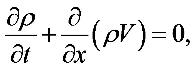
  and, some others. The number of macroscopic variables needed to understand the behavior varies according to the level of description we want to give. It should be noted that we consider all vehicles traveling in one direction, along a highway with one lane, this fact makes the problem one-dimensional. Also, we consider the motion in a closed circuit in order to have periodic boundary conditions. In this work we will consider three models [8,13,18], which share the structure of the balance equations for the relevant variables. First of all, we have the continuity equation for the density
 (1)
(1)
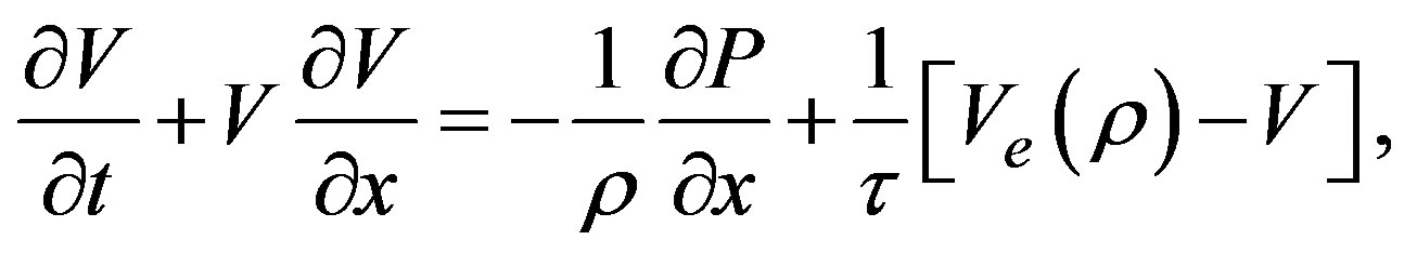
valid for the three models. The average speed satisfies a balance equation, in the case of models coming from a direct analogy with Navier-Stokes compressible fluid mechanics, such as the Helbing’s improved model (H) and the Kerner-Konhäuser model (K), it means
 (2)
(2)
where is the traffic pressure and
  the average relaxation time. In the case of the model called as Continuum Car-Following (CCF) it comes from a discrete traffic model, in such a case the speed equation shares the structure, but it cannot be written as in Equation (2) as emphasized in Section 4. Model H also considers the speed variance dynamics as relevant in the description, it has the structure of a usual balance equation and will be given afterwards. All these models have the contribution coming from the fundamental diagram
 , which represents the speed profile to which the drivers tend with a relaxation time given by
 . The fundamental diagram gives us a relation between the speed and the density when the system is in a homogeneous steady state. It considers all values between zero and their maximums in the speed and the density, meaning that such a relation exists even in the congested traffic region. It seems that this hypothesis is responsible for the lack of transition from free to synchronized phase
 , in GM models. The fundamental diagram, as well as the relaxation time are taken from the empirical observations. The models studied here will take the speed
  given by the fundamental diagram which tends to the maximum speed
  allowed in the highway at low densities and, tends to zero when the density is near the maximum density
  determined by the bumper-tobumper distance. In this work we will take the usual correlation for the fundamental diagram [8,9] which is given as
 (3)
(3)
where 
 ,
,  , with a maximum speed
  and the maximum density
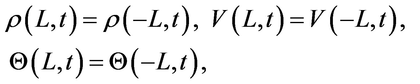
 . The boundary conditions to simulate the solution are taken as periodic
 (4)
(4)
they correspond to a closed circuit with a length given as . On the other hand, the initial conditions are chosen as follows
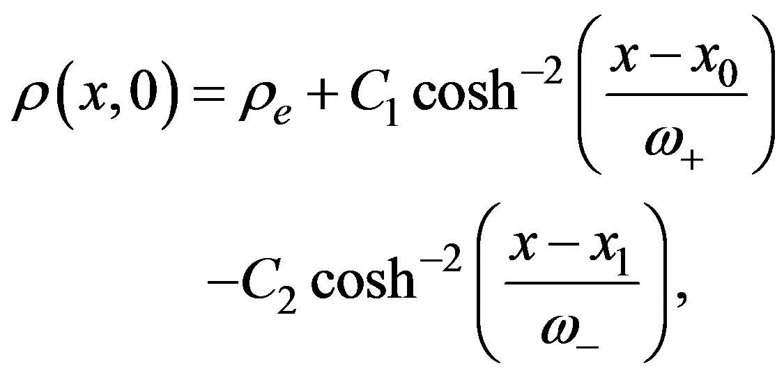 (5)
(5)
 (6)
(6)
where the constants  will be given for each illustrated case. The homogenous steady state determined by
  is a solution of the equations of motion in model H and, in the case of model K and CCF the corresponding state is given through
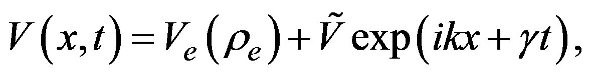
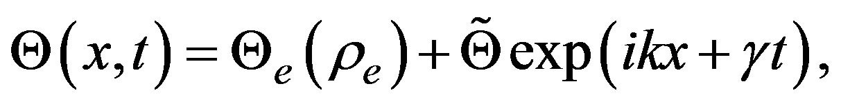
  The linear stability conditions associated to this state give us a way to begin the study of the mathematical properties contained in them. The linear stability conditions in these models are studied by means of a linearization of the equations of motion around the homogeneous steady state (called as the equilibrium state), then
 (7)
(7)
 (8)
(8)
 (9)
(9)
where  and
and  do not depend on position and time,
  is the wave vector and
  can be a complex function of the wave vector. The linear stability around the homogeneous steady state is granted when
 .The stability conditions determined in this way will be different for each model and they will be discussed in each particular case.
When the density  is chosen in the stable region, the perturbations around it decrease and the vehicles recover the homogenous steady state. On the other hand, if we are working in the unstable region, the perturbations grow and it is necessary to go into a deeper analysis.
3. Helbing’s Improved Model (H)
To begin our treatment, we consider the macroscopic model introduced by Helbing in 1995 [13] to overcome some difficulties presented by the Kerner-Konhäuser model [8,9]. In particular it was found that model K presents some problems concerning a density greater than the maximum value for certain parameter values. Instead of such behavior, the Helbing’s improved model does not have such undesirable properties. It shares the continuity and the speed equations with the Kerner-Konhäuser’s model, Equations (1)-(2). Model H also considers the speed variance  as a relevant variable and its evolution is determined by
 (10)
(10)
where the traffic pressure is proposed with a viscosity coefficient  and, a size correction for vehicles
  where
where  is the vehicle length and
  is the preferred headway of the driver, in such a way that
  represents a safe distance. These assumptions drive to a traffic pressure given as
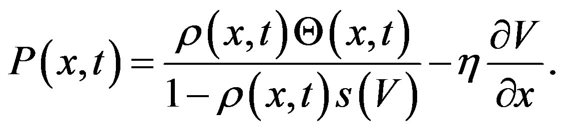 (11)
(11)
Notice that the traffic pressure resembles the corresponding Navier-Newton constitutive equation, where we have a term playing the role of the hydrostatic pressure, a viscosity coefficient with a size correction and, the speed gradient. On the other hand, the quantity  in Equation (10) represents the skewness in the speed distribution and can be seen as the analogous of the heat flow in compressible flow, it contains a kind of thermal conductivity coefficient
  and the size correction, they are given as follows
 (12)
(12)
the quantities and
and  are constants. It is worth noticing that the structure of the traffic pressure and
 , are very similar to the fluxes in usual fluid mechanics, however in traffic flow they do not have the same meaning. The finite size correction
  when
when  and, it has the effect to enhance the kinetic coefficients
  with a quantity which resembles the situation in a dense fluid. In contrast with Helbing’s work, in this paper the equilibrium variance
  is given through the variance prefactor
  and the fundamental diagram,
 (13)
(13)
the dimensionless variance prefactor is taken from correlations based on the empirical observations [29],
 (14)
(14)
where and
and  are constants.
Now, the homogeneous steady state is determined by  which are constants and satisfy the set of the equations of motion, as mentioned in Section 2. The linear stability analysis goes along the steps given in Equations (7)-(9). Also, the real parts in
  will determine the stability conditions, in fact, when
  we have stability. The real parts are developed in terms of the wave vector
  and the leading terms are given as follows,
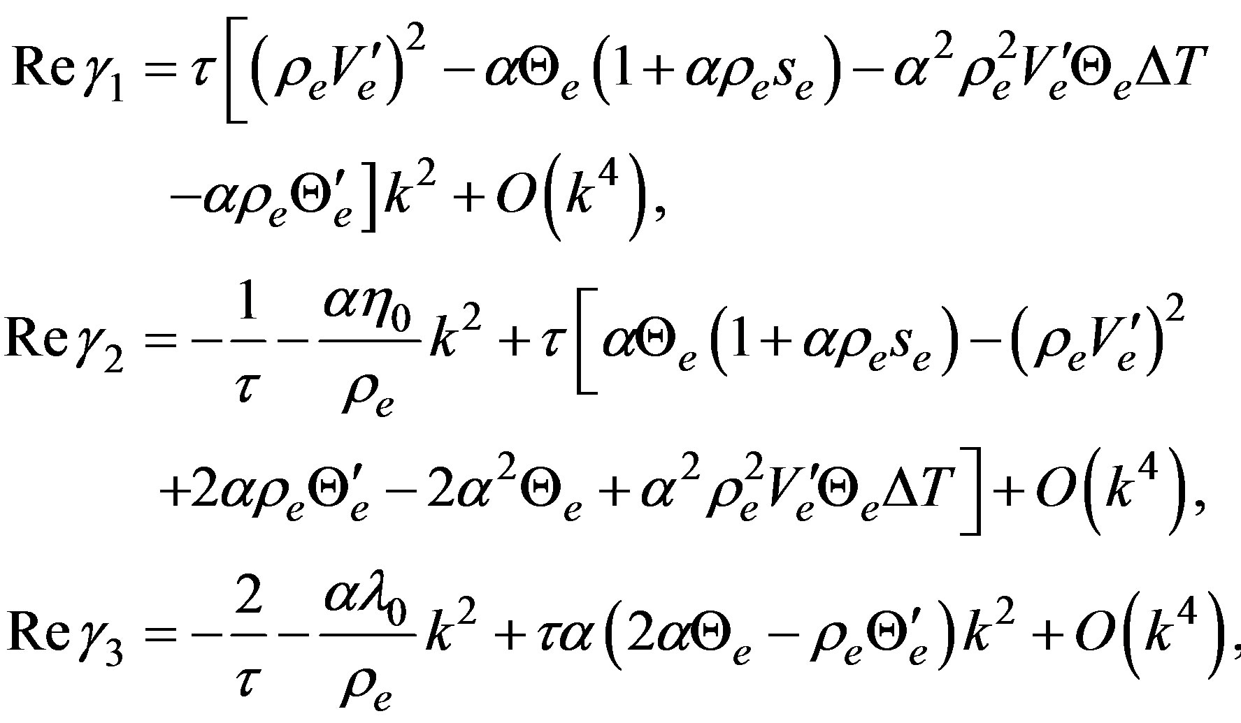 (15)
(15)
where we have written 
 and
and  to shorten the notation. The quantities
 are both related with the finite size of vehicles. On the other hand, the imaginary parts determine the speed of long wave length perturbations, they are given as
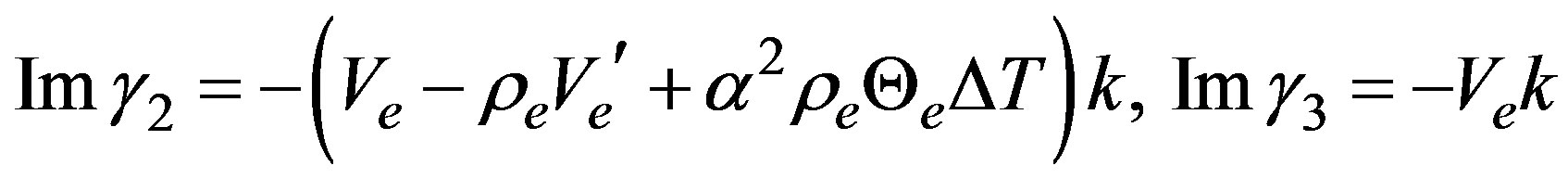 . Here the speed
  is given as
 (16)
(16)
and it is determined by the characteristics in the fundamental diagram. When we take the expression given in Equation (3), we can see that  can be positive or negative as a function of
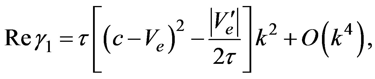
  The negative value of the imaginary parts for the three roots in Equation (15) is shown in Figure 1. Equations (15) deserve some comments, first of all, they were calculated up to second order in the wave vector, meaning that they are approximated and only the leading terms are given. Second, the leading term in the real part of root
  goes as
  and it must be negative to have stability in the equilibrium state, otherwise this state is unstable. Hence, the stability condition is written as
 (17)
(17)

Figure 1. Propagation speed of wavelength perturbations as functions of the density ρe, in model H. They are determined by the negative of the imaginary parts of roots γ1, γ2, γ3.
As a third comment, we notice that the real parts in roots  define a time scale proportional to
 , which does not tend to zero in the limit when
 . As a summary, the real parts in the dispersion relation roots, define two time scales in the problem, one of them determines the stability and the other one
  is given according to the model. When the stability condition is satisfied as an equality we obtain marginal stability.
In this model, the marginal stability reduces to a point corresponding to an equilibrium density
 . It means that for densities
 the homogeneous steady state is not linearly stable. In this point, it is important to emphasize that in model H, the homogeneous congested traffic state (HCT) is not present. This characteristic makes model H different from other GM models, where the stability region is bounded by a coexistence curve allowing a HCT state at high densities.
The simulation is done according to the expressions given in Section 2, with the following data 

 and the speed variance calculated according to Equations (13)-(14) is given by
 . Figure 2 shows the results for the density profile obtained with the two-step Lax-Wendroff method, after
  and
and  where it is permanent. The density profile corresponding to
  describes the transient behavior, whereas the profile in
  presents the structure of a wide moving jam in a highway. Figure 3 shows the typical behavior for the speed variance obtained from the numerical simulation.
It is important to notice that the density  chosen to implement the simulation corresponds to the linearly unstable region. As a result we have obtained a density profile in which the maximum density is less than

Figure 2. Density profile in Helbing’s improved model, dotted line is taken after t = 10.0 min and t = 100.0 min (full line) of simulation.
and the speed is always positive. This result means that once the perturbation has occurred it grows and then, after a transient time interval, a permanent density profile is obtained. Also, the presence of this profile indicates a cluster (J) formation propagating along the highway. The cluster speed measured shows that it remains constant, once the traveling wave has acquired its permanent profile. The data given in the simulation imply the existence of a cluster traveling upstream with a constant speed . Lastly, the characteristics of the cluster, such as the amplitude and width depend on the values taken for the model parameters, as will be shown in Section 6.
As a second example, in Figure 4 it is shown the temporal evolution of the density profile when  , which corresponds to a denser case in the unstable region. Also, the speed
  increases, the perturbation travels upstream and, the simulation results show
 . The density profiles taken at different times show the same qualitative behavior as in the case given before. However the permanent density profile becomes slightly wider than in the previous case. This result is clear taking into account that we have taken
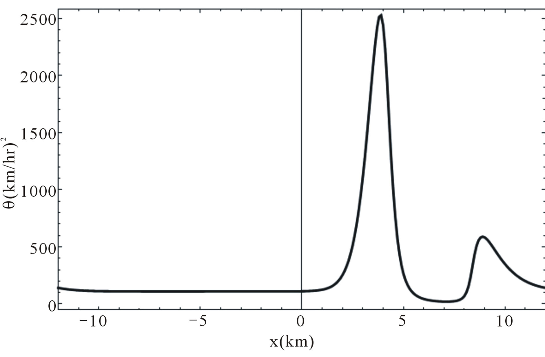
Figure 3. Typical behavior of the speed variance profile after t = 100.0 min, for a closed circuit of length L = 12 km.
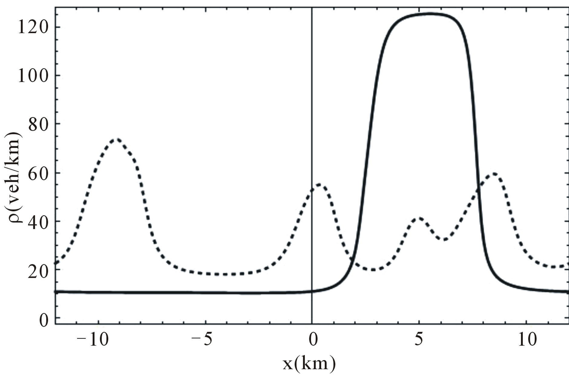
Figure 4. Temporal evolution of the density profile in the case ρe = 35.0 veh/km, the dotted line is taken at t = 10.0 min and the full line corresponds to t = 260.0 min.
a bigger value for .
.
4. Second Order Models (K, CCF)
Let us consider two macroscopic models which share the continuity and speed equations of motion, but do not consider the speed variance as determined by the dynamics.
4.1. The Kerner-Konhäuser Model (K)
In this model the traffic pressure is given according to a close analogy with fluid mechanics, in fact it corresponds to a particular case in model H. It is obtained when we neglect the size of vehicles, take a constant value for the speed variance,  in the traffic pressure and a viscosity
 . Then the traffic pressure is given as
 (18)
(18)
and it resembles to the Navier-Newton constitutive equation for a viscous fluid. In our case the coefficient  is the analogous of the bulk viscosity, due to the compressible character in the flow. The first term is the analogous of the hydrostatic pressure and, in this case is represented by the term
 .The direct substitution of the traffic pressure in Equation (2) gives us
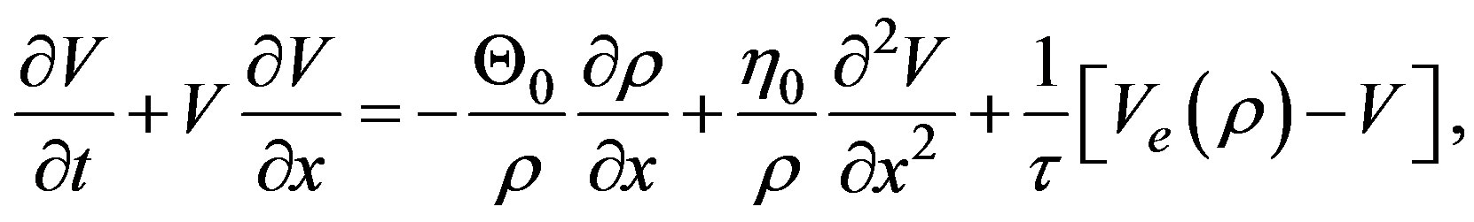 (19)
(19)
where we can see in a clear way the analogy with the Navier-Stokes equation. Notice that the speed variance is not taken as a relevant variable, then we only need two equations of motion to describe the system.
According to the stability considerations given in Section 2, we linearize the set of Equations (1), (19) around the equilibrium state and calculate the real parts of roots , hence
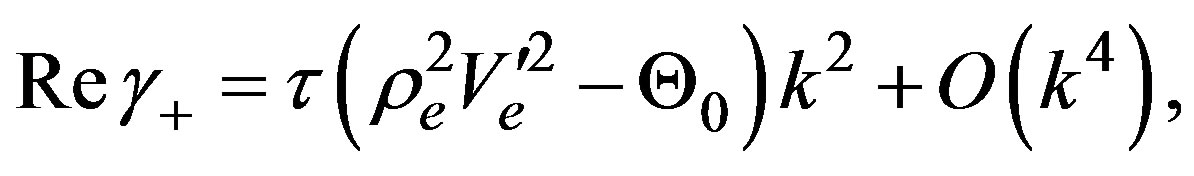 (20)
(20)
 . (21)
The imaginary parts of roots  to lowest order in the wave vector are given as
 , where
  gives us the propagation of long wave length perturbation waves, its behavior can be seen in Figure 1.
The results shown in Equations (20), (21) show us immediately that in this model there exist two time scales, one is determined by the relaxation time  and the other one depends on the fundamental diagram and the value for the variance
 . Besides they depend on the wave vector. In fact, Equation (20) determines the marginal stability and it contains the reference density
 , in such a way that we can consider a kind of coexistence curve which separates the space determined by
  in stability regions. Figure 5 shows the coexistence curve determined by the condition (marginal stability)
 the stability region corresponds to
 and it is located outside the curve. This figure shows in a clear way that model K allows the existence of HCT states. It is important to notice that the roots
  are given to leading orders in the wave vector
 .
.
As a second step in the K model analysis, we recall that the stability regions are determined within the frame on the linearization of the equations of motion. It means that beyond the linear regime, this analysis cannot be taken. In fact, the present instabilities do not show themselves when we simulate the complete model, even when we work around densities  chosen in the unstable region.
The numerical simulation of this model starts with the initial conditions shown in Equations (5), (6) with  ,
,
 and the equilibrium density
  in the unstable region when
 . Also, we take periodic boundary conditions for the density and the speed, as given in Equation (4). Figure 6 shows the results for
  and
and  respectively. We observe that after a transient, the density presents a permanent profile representing an upstream traveling wave with constant speed given as
 .
.
In all cases the speed and density profiles are coupled closely. The maximum (minimum) in density corresponds to a minimum (maximum) in the speed.
4.2. Continuum Car-Following Model (CCF)
There are several microscopic models to study traffic flow, one of the most common class corresponds to the
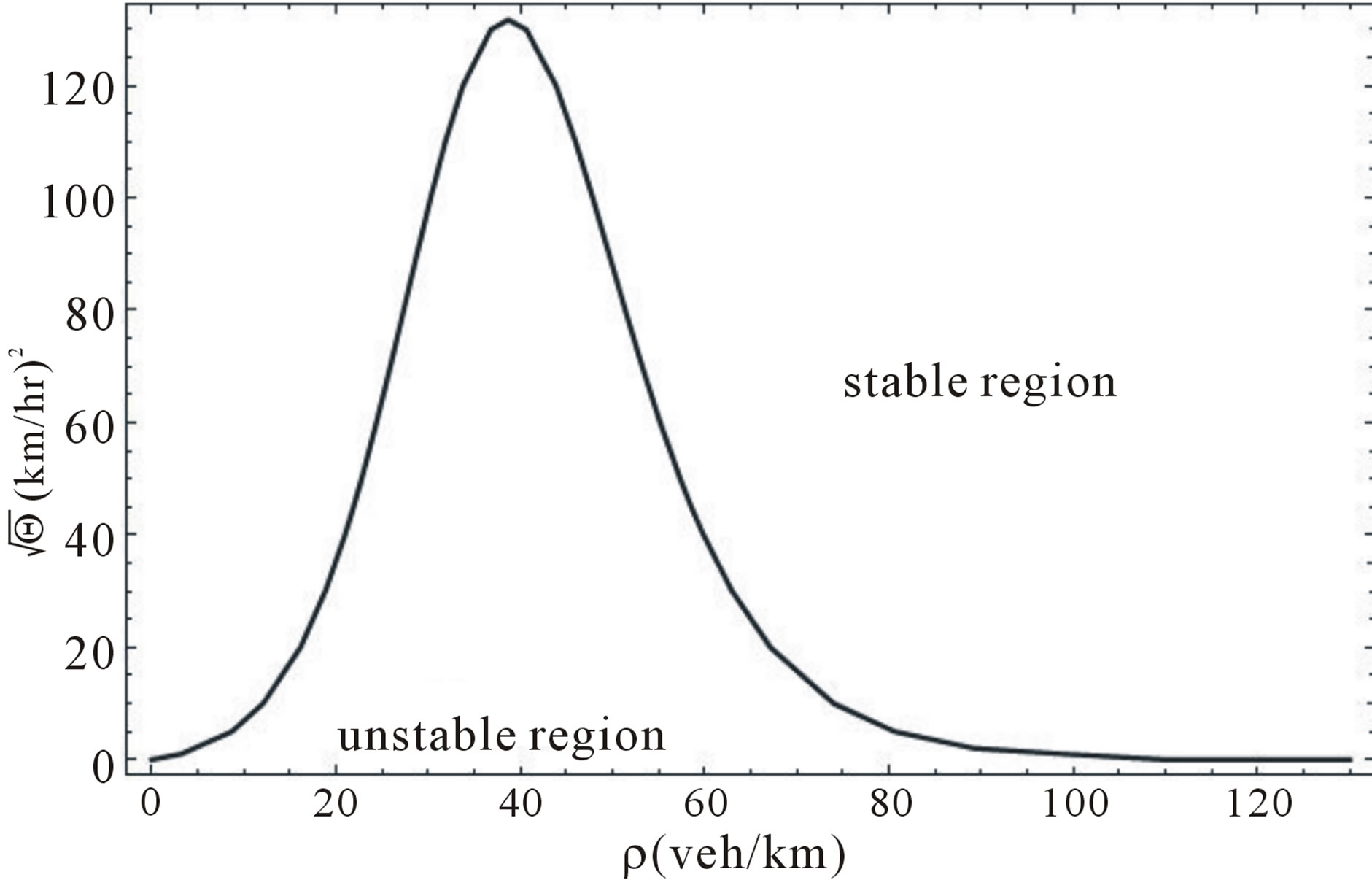
Figure 5. Stability regions in the Kerner-Konhäuser model. The maximum speed allowed in the highway is taken as Vmax = 120 km/h and the maximum density is taken as ρmax = 140 veh/km and, Θ0 = (45.0 km/h)2, τ = 30 s.

Figure 6. Temporal evolution of the density profile in model K, the dotted line gives the profile for t = 10.0 min and the full line represents the permanent profile after t = 100.0 min, ρe = 28.0 veh/km, τ = 0.5 min.
car-following structure. Though these models follow each vehicle while they are moving, Berg, et al. [18] constructed their continuum version. The main idea behind this method was to write the headway in terms of the density and its derivatives. With such a method it is possible to write the average speed equation as a continuum equation, which is given as
 (22)
(22)
where we have written the relaxation time  instead of the sensibility factor
  as it is usual in this model. Equation (22) can also be written in a similar way as the Navier-Stokes equation,
 (23)
(23)
In contrast with the model K, now we have density dependence in the term equivalent to the hydrostatic pressure while the viscosity term depends on the density gradient instead of the speed gradient. In spite of these differences, the structure of the equation contains the same characteristics as Equation (19). The linear stability analysis can be done with the same procedure to obtain
 (24)
(24)
 (25)
(25)
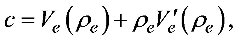
where it is shown the two time scales and quantity  is given in Equation (16). Consequently we also have a coexistence curve separating the space according to the stability characteristics. Figure 7 shows the regions in the space
 . On the other hand, the imaginary part of roots
  determines the propagation speed of long wave length perturbations and, they are given as
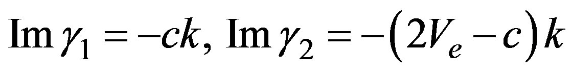 . Later on we will show that this model presents the same qualitative behavior as model K, due to the existence of the two time scales we have found in Equations (24), (25).
We remark that models K and CCF have a coexistence curve which bounds the instability region. Stability occurs outside the marginal stability curve shown in Figures 5, 7 giving place to the HCT states at the high density region.
5. The Iterative Method
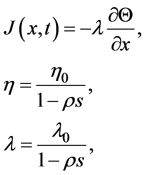
A way to go further in the search for an explanation to this behavior, is provided by the method proposed by Berg and Woods [18]. By means of an iterative procedure it is possible to calculate approximately the flux defined as  this method allows the identification of a traveling wave with the properties of a soliton. The main idea behind the approximation is based on the existence of several time scales in the problem [31]. In particular, the three models we have presented have two time scales given through the relaxation time
  and the characteristics in the fundamental diagram. Those time scales are separated clearly due to the fact that one of them is determined by experimental data and the other has a
  dependence. Now, let us apply the iterative procedure to the models presented above.
To begin the procedure, the equations of motion (1, 2, 22, 10) are written in a reference frame moving with constant speed . We introduce the variable
  and, all derivatives will be indicated with a sub index
 . The continuity equation is then written as
 (26)
(26)
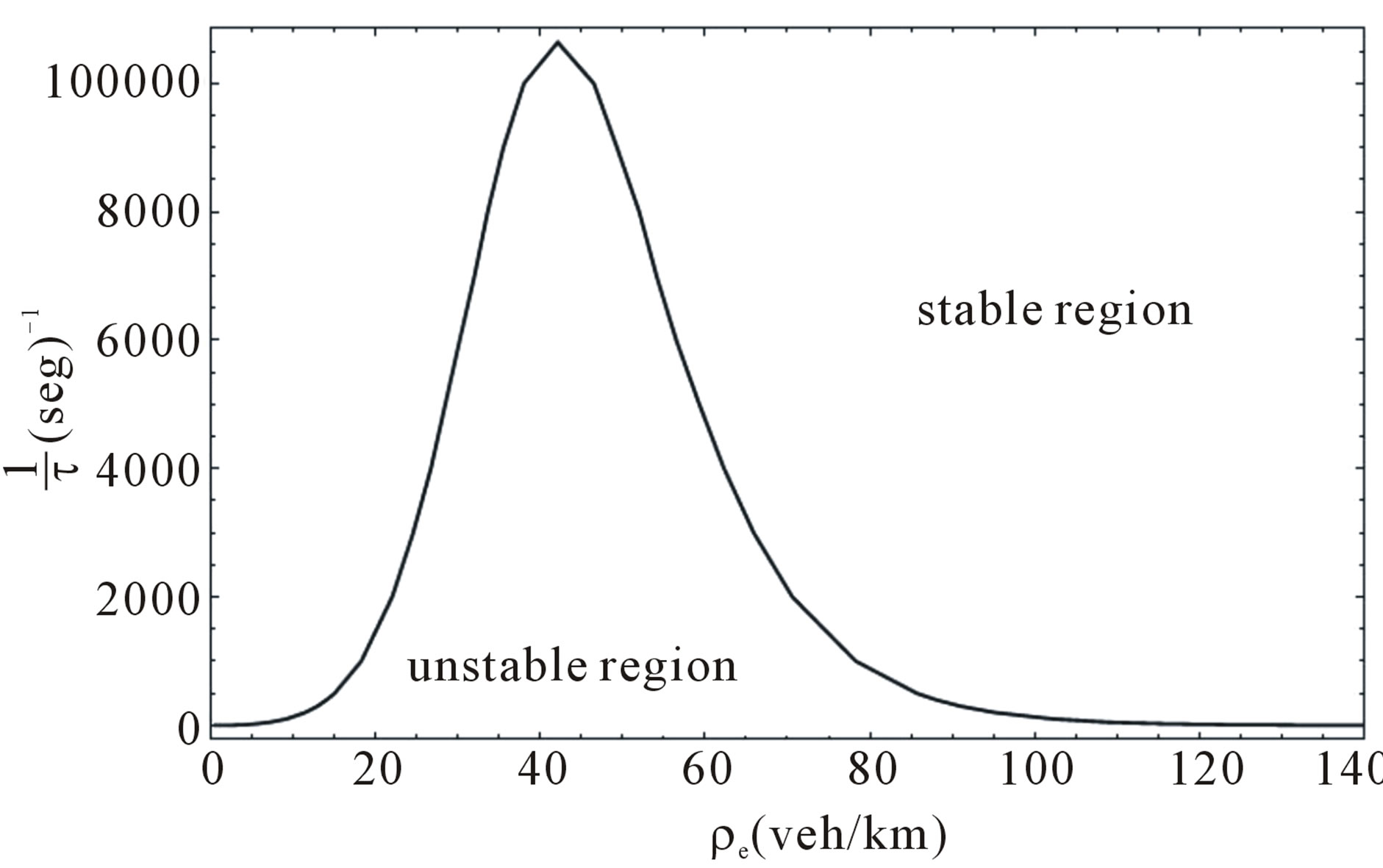
Figure 7. Coexistence curve for the continuum car-following model.
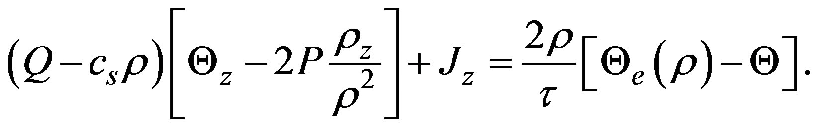
which can be integrated, the speed Equation (2) is written in terms of the flux 
 (27)
(27)
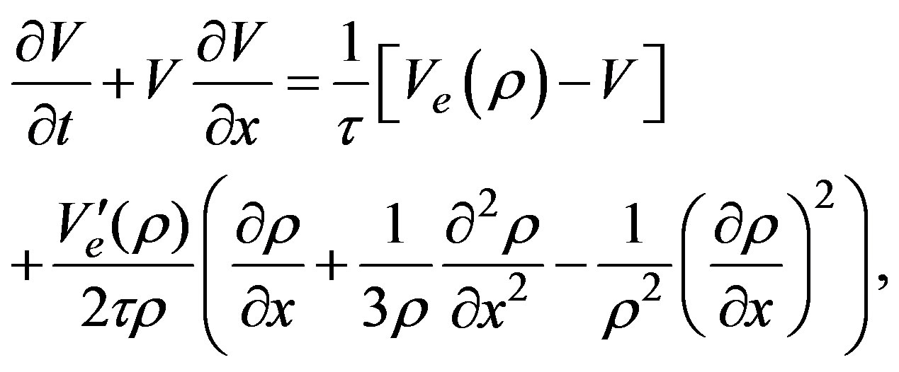
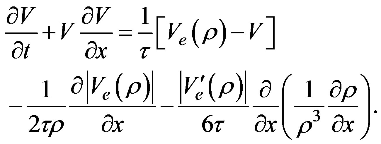
where in agreement with the continuity Equation (26). We recall that Helbing and Kerner-Konhäuser’s models share the structure of the speed equation, the difference between them is given through the traffic pressure expressions. In a similar way, the speed equation in the continuum car-following method Equation (23) is also written in the new reference frame,
 (28)
(28)
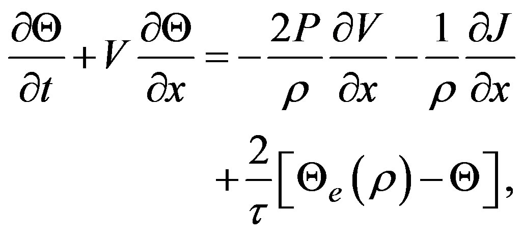
lastly, the speed variance equation is written as
 (29)
(29)
The first step in the iterative process is done with the consideration of a solution up to order zero in the  -derivatives. It is clear that this solution is given as
 (30)
(30)
To continue in a clear way, let us consider first the Helbing’s model where the  -derivative for the traffic pressure is given as
 (31)
(31)
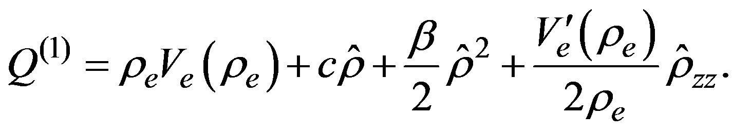
The substitution of Equation (31) in the left hand side of Equation (27) gives us a value for the first order iteration in the flux,
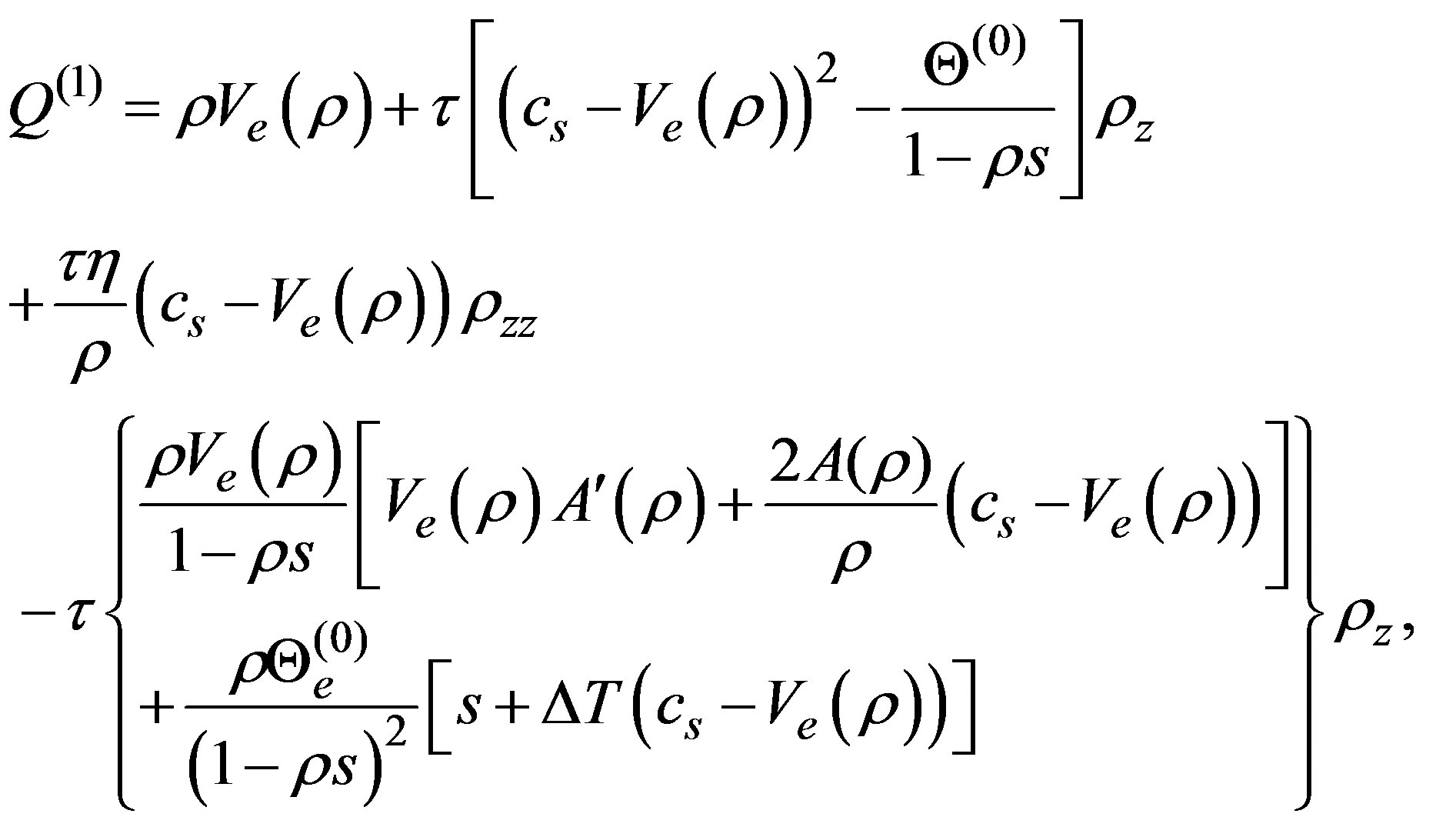 (32)
(32)
where the bilinear or quadratic terms like  have been neglected to this order. Now, the speed
  given according to the fundamental diagram is developed around the equilibrium density
  up to second order terms,

and we have called the density deviation as .
.
The direct substitution of Equation (32) and the  expansion in Equation (26) drives us to,
 (33)
(33)
where  is given in Equation (16) and
 (34)
(34)
is determined in terms of the fundamental diagram and the speed . It should be noted that Equation (33) does not represent the complete solution as described in the simulation, instead it is an approximation of the model in which some small terms have been neglected. For example, the fundamental diagram contains terms of all order in
 , there are derivatives of higher order than the ones considered in this approximation, also, some nonlinear terms in the derivatives are neglected. Equation (33) is the well known Korteweg-de Vries (KdV) equation for the density
  when written in the moving reference system
  [30]. The simplest solution can be found immediately and it is given as,
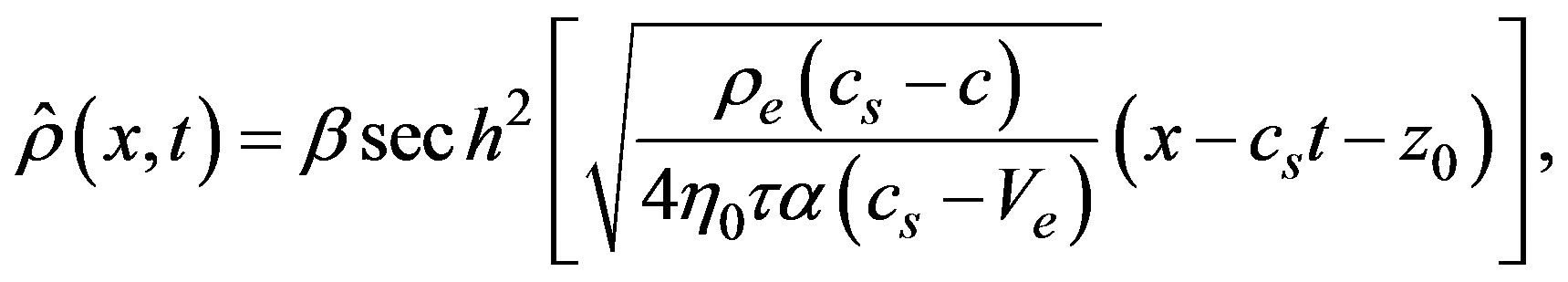 (35)
(35)
where we recall that the quantities  are evaluated in the density
 , besides
 . This solution is obtained by means of direct integration and two integration constants are taken as zero. The quantity
  corresponds to an integration constant and it is interpreted as the soliton center. Obviously, the soliton amplitude is given by
  and it must be positive. Also, the quotient
  must be positive, when both conditions are valid simultaneously, they guarantee that the soliton amplitude be positive and the width a real quantity, as we will see soon.
We now apply the same method to model K, taking the speed Equation (28) we find the first order approximation in the flux,
 (36)
(36)
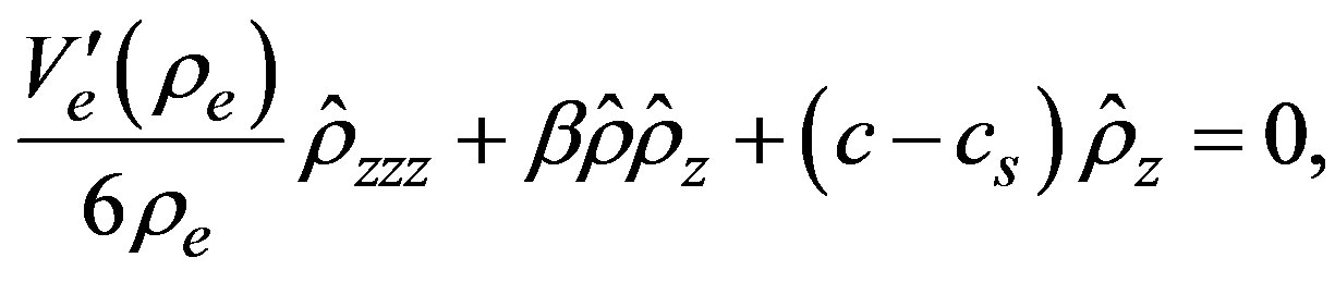
Also, we have neglected second order terms in the  -derivatives. Now, we follow the same steps as in model H and find the corresponding KdV equation in this case,
 (37)
(37)
which is essentially the same equation as in model H, the only difference being the presence of the vehicle size and safe distance as represented by .
.
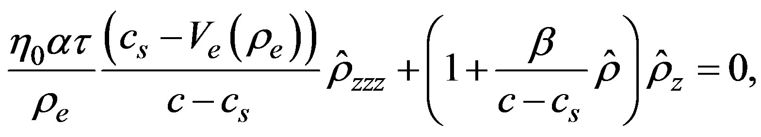
Now, let us consider the set of Equations (26), (27) in the case corresponding to the CCF model. The iterative procedure follows the same steps to obtain the first order correction to the flux, the result is given as,
 (38)
(38)
The procedure described above is applied to obtain the evolution of the density in the moving reference frame, so
 (39)
(39)
where  is given before. Equation (39) represents a soliton with the same structure as given in Equation (33) with some differences to be compared later.
Lastly, the variance corresponding to model H in this approximation can be written as
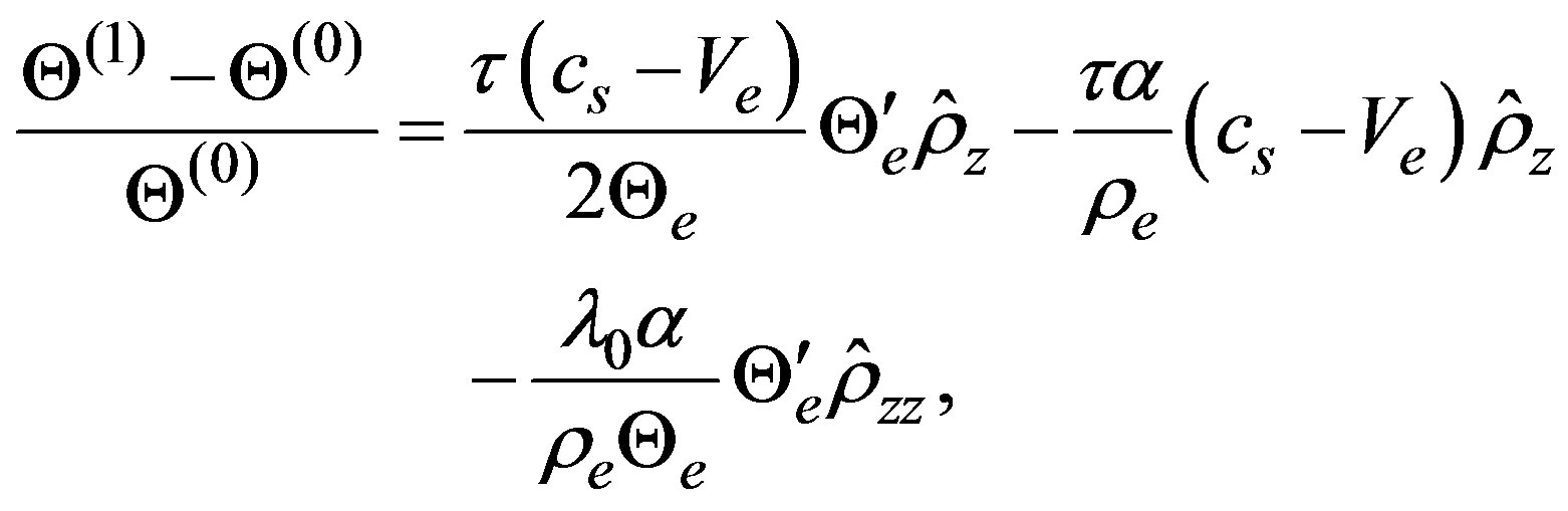 (40)
(40)
and we notice that it is not coupled with other quantities but the deviation in the density.
6. Soliton Characteristics
To compare the results obtained with the three models, let us define the soliton width, with respect to its center, and in terms of the density profile along the highway length,
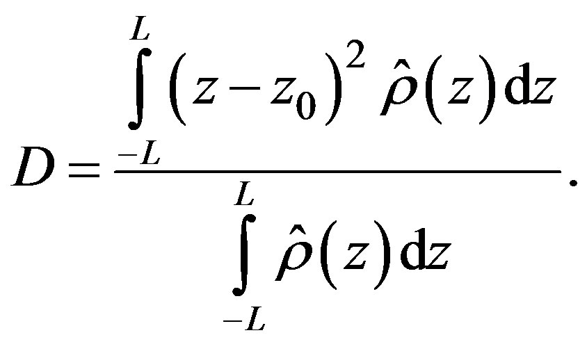 (41)
(41)
This quantity can be calculated for the three models and the results are shown in the following table.
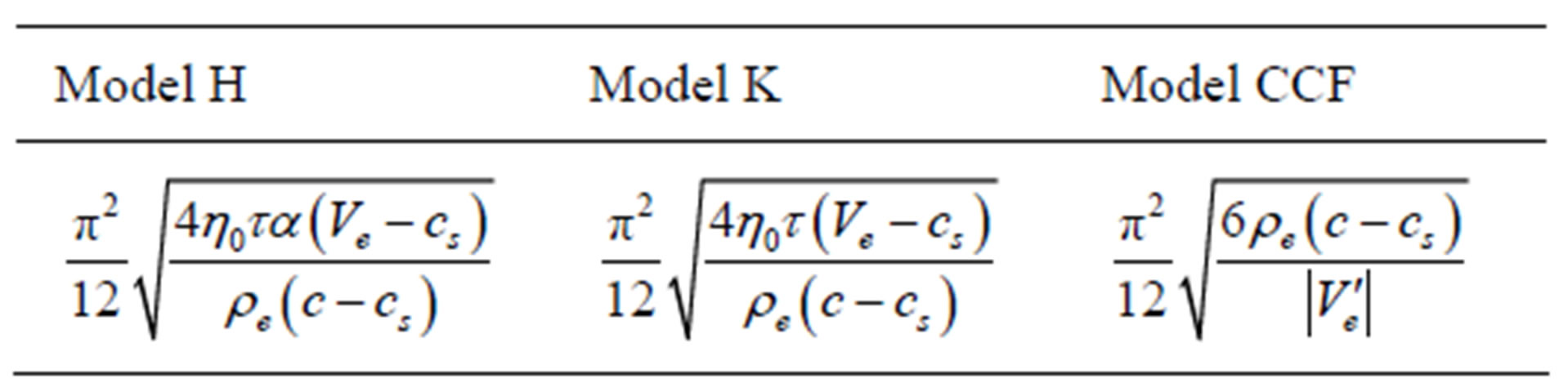
All of them look very similar however, they contain explicitly the parameters introduced by the model itself, the speed  corresponding to the traveling wave and, the characteristics in the fundamental diagram. Notice that model H contains the size of vehicles and the safe distance through the quantity
 . Figure 8 shows the comparison between them, for a given constant
  As we mentioned before the KdV solution must satisfy certain conditions in order to have a physical solution to be realized in traffic flow. In particular, we must ask the amplitude be a positive quantity and the width must be real. Due to the fact that these quantities are functions of the model parameters and the fundamental diagram, we can observe that it may exists some regions for which the soliton solution is not a valid one. On the other hand, the sign of the amplitude in models H and K depends on a quotient between the propagation speed of long wavelength perturbations as referred to
  and given by Equation (16), which can be positive or negative according to the density value
 . Besides, in the denominator there is a combination of terms depending on the fundamental diagram. Also, the width depends on a similar combination of quantities, hence it is possible to construct a line which divides the plane
  in regions where the soliton exists. Figure 9 shows those regions for H and K models.
width (km)
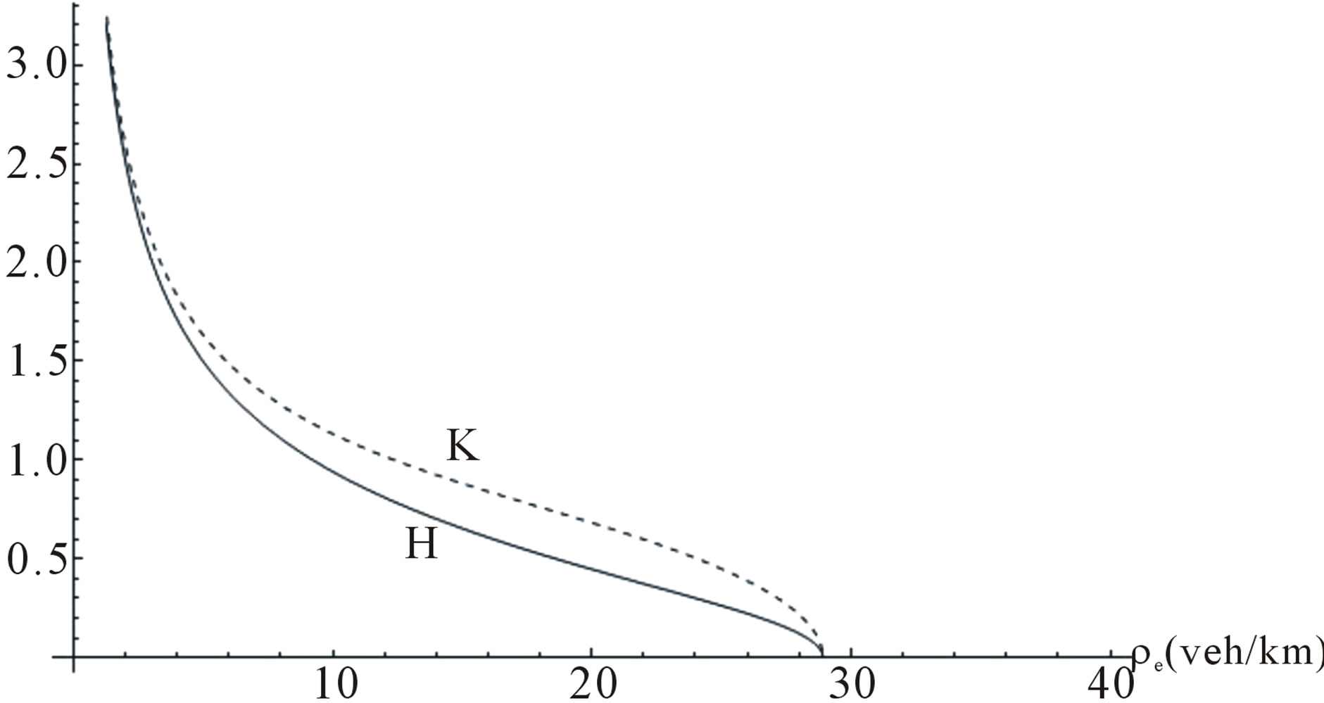
Figure 8. Comparison between the soliton widths for models H and K. The speed cs = –10 km/h.
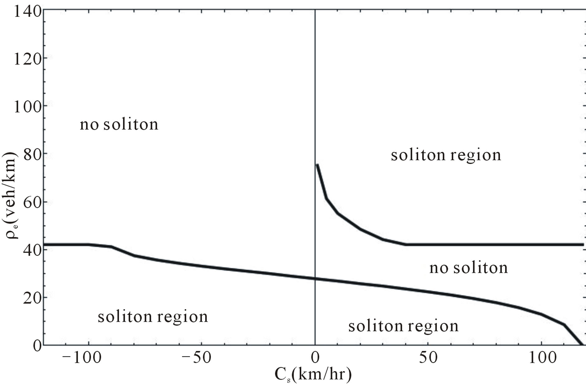
Figure 9. The curve shows the separation between regions where it is possible to find a soliton solution in model H and K.
The regions where the soliton solutions exist change according to the value of the equilibrium density  and the soliton speed
 , which is the speed of the reference frame. In fact, the simulation results show the
  meaning that the cluster travels upstream. In Figure 9 we have drawn the complete region for
  and we can observe that in the case when
  the plane presents two regions where the soliton can be formed and a region where it is not. It means that the cluster can be formed for certain equilibrium densities, when the cluster travels downstream. In contrast, when
  there is a maximum density
  for which the cluster exists. Notice that models H and K share this characteristic, a fact which is explained with the observation that the conditions for the existence of the cluster are the same in both models.
In a similar way we can construct the line allowing the soliton existence in the CCF model, where we see that there is only one line separating regions and, the soliton can travel upstream or downstream. Figure 10 shows the corresponding line in plane .
.
7. Concluding Remarks
The macroscopic modeling approach to traffic flow has shown to reproduce some characteristics of the behavior of vehicles in a highway. In particular, the model H does not present the HCT state in contrast to models K and, CCF. The three models take the same fundamental diagram and in the linearly unstable region allow the formation of clusters which can be seen as wide moving jams (J). Besides the properties shown in the numerical simulation, the iterative procedure has allowed us to find, in an analytical way, the approximate structure of such clusters. Numerical calculations have been done to show this behavior in microscopic models, however, it is interesting to show that models including the size of vehicle behave in the same way. Certainly, the calculation is an approximate one, but it gives the qualitative properties of the clusters. The comparison between these models
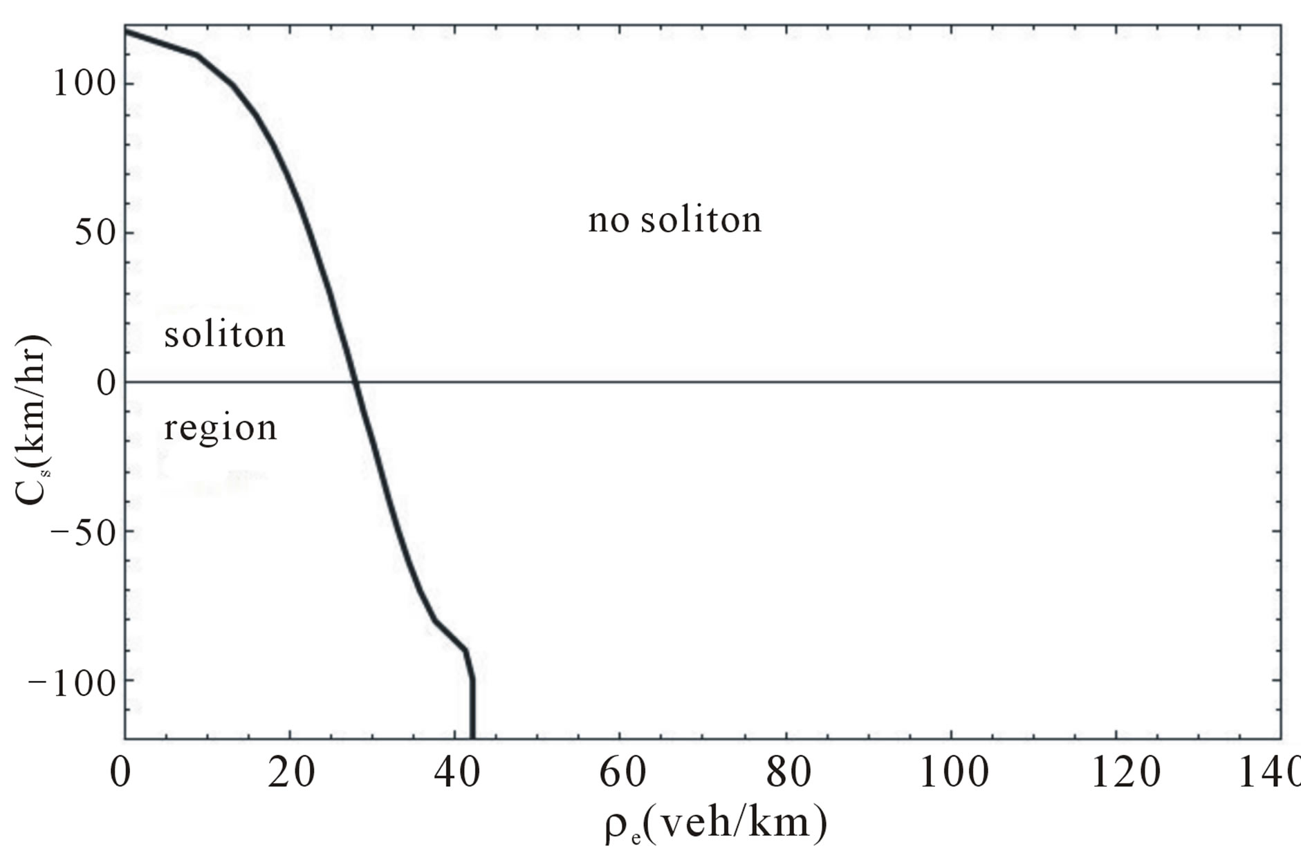
Figure 10. Separation line for model CCF.
has shown that the macroscopic analogy with compressible fluid mechanics is fruitful to understand some characteristics in traffic.
REFERENCES
- H. X. Ge, R. J. Cheng and S. Q. Dai, “KdV and KinkAntikinksolitons in Car-Following Models,” Physica A: Statistical Mechanics and Its Applications, Vol. 357, No. 3-4, 2005, pp. 466-476. doi:10.1016/j.physa.2005.03.059
- H. B. Zhu and S. Q. Dai, “Numerical Simulation of Soliton and Kink Density Waves in Traffic Flow with Periodic Boundaries,” Physica A: Statistical Mechanics and Its Applications, Vol. 387, No. 16-17, 2008, pp. 4367- 4375. doi:10.1016/j.physa.2008.01.067
- Z. Z. Liu, X. J. Zhou, X. M. Liu and J. Luo, “Density Waves in Traffic Flow of Two Kinds of Vehicles,” Physical Review E, Vol. 67, No. 1, 2003, pp. 017601-017604. doi:10.1103/PhysRevE.67.017601
- D. Helbing, “Traffic and Related Self-Driven Many-Particle Systems,” Reviews of Modern Physics, Vol. 73, No. 4, 2001, pp. 1067-1139. doi:10.1103/RevModPhys.73.1067
- M. J. Lighthill and G. B. Whitham, “On Kinematic Waves II. A Theory of Traffic Flow on Long Crowded Roads,” Proceedings of the Royal Society of London, Vol. 229, 1955, pp. 317-345.
- H. J. Payne, “Mathematical Models of Public Systems,” Simulation Councils, Inc., 1971.
- R. D. Kühne and R. Beckschulte, “Transportation and Traffic Theory,” Proceedings of 12th International Symposium on Transportation and Traffic Theory, Elsevier, Berkeley, 1993.
- B. S. Kerner and P. Konhäuser, “Cluster Effect in Initially Homogenous Traffic Flow,” Physical Review E, Vol. 48, No. 4, 1993, R2335-R2338. doi:10.1103/PhysRevE.48.R2335
- B. S. Kerner and P. Konhäuser, “Structure and Parameters of Clusters in Traffic Flow,” Physical Review E, Vol. 50, No. 51, 1994, pp. 54-83. doi:10.1103/PhysRevE.50.54
- A. Aw and M. Rascle, “Resurrection of “Second Order,” Models of Traffic Flow,” SIAM Journal of Applied Mathematics, Vol. 60, No. 3, 2000, pp. 916-938. doi:10.1137/S0036139997332099
- A. Aw, A. Klar, T. Materne and M. Rascle, “Derivation of Continuum Traffic Flow Models from Microscopic Follow the Leader Models,” SIAM Journal of Applied Mathematics, Vol. 63, No. 1, 2002, pp. 259-278. doi:10.1137/S0036139900380955
- W. Marques Jr. and R. M. Velasco, “An Improved Second-Order Continuum Traffic Model,” Journal of Statistical Mechanics: Theory and Experiment, Vol. 2010, 2010, P02012. doi:10.1088/1742-5468/2010/02/P02012
- D. Helbing, “Improved Fluid-Dynamic Model for Vehicular Traffic,” Physical Review E, Vol. 51, No. 4, 1995, pp. 3164-3169. doi:10.1103/PhysRevE.51.3164
- D. Helbing, “Theoretical Foundation of Macroscopic Traffic models,” Physica A: Statistical Mechanics and Its Applications, Vol. 219, No. 3-4, 1995, pp. 375-390. doi:10.1016/0378-4371(95)00174-6
- C. Wagner “Second-Order Continuum Traffic Flow Model,” Physical Review E, Vol. 54, No. 5, 1996, pp. 5073-5085. doi:10.1103/PhysRevE.54.5073
- R. M. Velasco and W. Marques Jr., “Navier-Stokes-Like Equations for Traffic Flow,” Physical Review E, Vol. 72, No. 4, 2005, pp. 046102-046110. doi:10.1103/PhysRevE.72.046102
- A. R. Méndez and R. M. Velasco, “An Alternative Model in Traffic Flow Equations,” Transportation Research Part B, Vol. 42, No. 9, 2008, pp. 782-797. doi:10.1016/j.trb.2008.01.003
- P. Berg and A. Woods, “On-Ramp Simulations and Solitary Waves of a Car-Following Model,” Physical Review E, Vol. 64, No. 3, 2001, 035602(R). doi:10.1103/PhysRevE.64.035602
- D. Helbing and M. Treiber, “Numerical Simulation of Macroscopic Traffic Equations,” Computing in Science & Engineering, Vol. 1, No. 5, 1999, pp. 89-99. doi:10.1109/5992.790593
- Y. Sugiyama, M. Fukui, M. Kikuchi, K. Hasebe, A. Nakayama, K. Nishinari, S. Tadaki and S. Yukawa, “Traffic Jams without Bottlenecks-Experimental Evidence for the Physical Mechanism of Formation of a Jam,” New Journal of Physics, Vol. 10, No. 3, 2008, 033001. doi:10.1088/1367-2630/10/3/033001
- B. S. Kerner, “The Physics of Traffic,” Springer, Berlin, 2005.
- B. S. Kerner, “Introduction of Modern Traffic Flow Theory and Control,” Springer, Berlin, 2009. doi:10.1007/978-3-642-02605-8
- B. R. Kerner, “Enciclopedia of Complexity and Systems Science,” Springer, Berlin, 2009, pp. 9302-9355.
- P. Berg, A. Mason and A. Woods, “Continuum Approach to Car-Following Models,” Physical Review E, Vol. 61, 2000, pp. 1056-1066. doi:10.1103/PhysRevE.64.035602
- D. A. Kürtze and D. C. Hong, “Traffic Jams, Granular Flow, and Soliton Selection,” Physical Review E, Vol. 52, No. 1, 1995, pp. 218-221. doi:10.1103/PhysRevE.52.218
- P. Saavedra and R. M. Velasco, “Solitons in a Macroscopic Traffic Model,” 12th IFAC Symposium on Transportation Systems, 2009, pp. 428-433.
- R. M. Velasco and P. Saavedra, “Clusters in the Helbing’s Improved Model,” Lecture Notes in Computational Science 6350, 2010, pp. 633-636.
- M. Treiber and D. Helbing, “Macroscopic Simulation of Widely Scattered Synchronized Traffic States,” Journal of Physics A: Mathematical and General, Vol. 32, No. 1, 1999, pp. L7-L23. doi:10.1088/0305-4470/32/1/003
- V. Shevtsov and D. Helbing, “Macroscopic Dynamics of Multilane Traffic,” Physical Review E, Vol. 59, No. 6, 1999, pp. 6328-6338. doi:10.1103/PhysRevE.59.6328
- P. G. Drazin and R. S. Johnson, “Solitons: An Introduction,” Cambridge University Press, Cambridge, 1990.
- R. S. Johnson, “Singular Perturbation Theory,” Springer, Berlin, 2004.