International Journal of Astronomy and Astrophysics
Vol.3 No.4(2013), Article ID:40324,9 pages DOI:10.4236/ijaa.2013.34047
Estimation of Magnetospheric Plasma Parameters from Whistlers Observed at Low Latitudes
1Department of Physics, National Institute of Technology, Srinagar, India
2Department of Civil engineering, National Institute of Technology, Srinagar, India
Email: altafnig@rediff.com
Copyright © 2013 Mohd Altaf et al. This is an open access article distributed under the Creative Commons Attribution License, which permits unrestricted use, distribution, and reproduction in any medium, provided the original work is properly cited.
Received March 22, 2013; revised April 20, 2013; accepted April 28, 2013
Keywords: Magnetosphere; Electron Temperature; Electric Field; Electron Density
ABSTRACT
Whistler observations during nighttimes made at low latitude Indian ground stations Jammu (geomag. lat., 29˚26'N; L = 1.17), Nainital (geomag. lat., 19˚1'N; L = 1.16) and Varanasi (geomag. lat., 14˚55'N; L = 1.11) are used to deduce electron temperatures and electric field in the vicinity of the magnetospheric equator. The accurate curve fitting and parameter estimation technique are used to compute nose frequency and equatorial electron densities from the dispersion measurements of short whistlers recorded at Jammu, Nainital and Varanasi. In this paper, our aim is to estimate the Magnetospheric electron temperatures and electric field from the dispersion analysis of short whistlers observed at low latitudes by using different methods. The results obtained are in good agreement with the results reported by other workers.
1. Introduction
It is well known that lightning discharges are accompanied by the generation of electromagnetic waves in a wide frequency range [1,2]. Wave energy can penetrate into the magnetosphere and propagate almost along geomagnetic field lines to the opposite hemisphere where it is recorded by a radio receiver called whistler. The dynamic spectrum of the recorded signal is typically dispersed in the spectrogram. These signals sometimes proceeded by an associated signal with an undispersed dynamic spectrum and are generated during the same lightning discharges but propagate in the Earth-ionosphere waveguide [2,3]. When this signal is recorded and coincides approximately with the moment of lightning discharge, its time delay does not usually exceed 0.04 s [4] as the velocity of wave propagation in the Earth-ionosphere waveguide is close to velocity of light, this signal is called an atmospheric or sferic. The whistler signal intensity is normally greatest at few kHz within the ELF/ VLF band; 1 - 20 kHz (Carpenter, 1962).
Whistlers represent an inexpensive and effective method for obtaining various plasmaspheric parameters like electron density, electron temperature, electric field etc. in the magnetosphere, but the experimental results published up to now refer mainly to higher latitudes [5-7], and a systematic description of the main features of the plasmaspheric electron density based on large quantities of whistler data is still lacking at high latitudes, with the exception of work by Park et al. [8]. Recently Tracsai et al. [9] have processed whistlers recorded at Tihany, Hungary (L = 1.9) between December 1970 and May 1975 in order to study the distribution of equatorial electron density and total electron content in flux tubes having Lvalue, lying in the range L = 1.4 - 3.2. At low latitudes, the exploration of whistlers for electron density determination has only been carried out by Lalmani et al. [10]. In this paper the equatorial electron density, equatorial electron temperature and east-west component of electric field at low latitudes using the whistler data observed at our ground stations Jammu, Nanital and Varanasi have been estimated.
At middle and high latitudes, both satellite and groundbased whistler data were exploited fully to reveal new facts about the structure and dynamics of the ionosphere and magnetosphere. These achievements included the discovery of the plasmasphere, plasmapause, and bulge [11], identification of the mechanism of ionosphere-protonosphere coupling [5,12] and the measurement of the magnetospheric electric field [13]. Although the application of whistlers to diagnostic of electron temperature of high latitudes has been discussed since the early 1960s [6,14,15], this problem still seems to be at an early stage of its development at low latitudes. At low latitudes, whistler data have been used for determining electron temperatures, electric field etc. for understanding the magnetospheric phenomena.
We consider the methods of “traditional” diagnostics of magnetospheric parameters, such as electron plasma density, the large scale electric field and possible temporal variations of the magnetic field at the magnetospheric equator, when both fn and tn are known. When one or both of these parameters are not known the dynamic spectra of whistlers and/or sferics need to be extrapolated. Method of this extrapolation is subsequently considered. Then we estimate the equatorial electron density, electron temperature, and electric field in the equatorial magnetosphere based on the analysis of the dynamic spectra of whistlers. Whistler studies in India, which have been in progress since 1963, have made significant contribution to the propagation of low latitude whistlers and understanding of the structure and dynamics of the low latitude ionosphere [16-18].
For the analysis of non-nose whistlers, a number of methods have been proposed [19]. The nose frequency of the whistler data used in estimating electron density, electron temperature and electric field has been computed by means of accurate curve fitting method developed by Tarcsai [19] based on least squares estimation of the two parameters, zero frequency dispersion Do, equatorial electron gyrofrequency fHe in Bernard’s approximation. This matched filtering technique developed for the analysis of whistler waves increases the accuracy of analysis and speed of data processing [17,18,20]. The technique employs dispersive digital filters whose frequency-time response is matched to the frequency-time response of the signal to be analyzed. Due to high resolution and time domain, many fine structure components with amplitudes differing in frequency and time are seen in dynamic spectra [20]. The accuracy and effectiveness of the technique have been discussed at length by analyzing a large number of whistlers both on the ground stations (from the low to the high latitudes) and onboard rockets/satellites [18,20-22].
Electric fields are closely related to and control most of observed gyophysical phenomena such as the bulk motion of the magnetospheric plasma, the current systems in the magnetosphere and the ionosphere, and to the acceleration of plasma particles in the Earth’s magnetosphere. The role of the electric field in controlling the bulk motion of the plasma has been recognized in all the theoretical studies of the various dynamic processes taking place in the Earth’s magnetosphere although adequate experimental techniques for the precise measurements of such fields in the ionosphere and magnetosphere were not available for quite some time. The observed cross-L motions of the whistler ducts are being used currently for obtaining the east-west component of the electric fields in the plasmasphere during substorm periods as well as quiet times [4,5].
The tidal forces in the Earth’s atmosphere cause motion of the plasma across the magnetic field lines and give rise to electromotive forces. The generation of electric field by the motion of conducting plasma across the magnetic field is analogous to dynamo action and the theory dealing with the electric field generation by this mechanism is known as dynamo theory. The electric field generation mechanism in the ionosphere has been developed by various workers [23,24]. Electric field measurements have been carried out in the equatorial Eregion of the ionosphere by many workers. These measurements reveal the existence of east-west electrostatic field raging from 1 to 2 mV/m. The whistler method of obtaining the east-west component of the electric field has the advantage of extended time coverage and remarkable property of being directly involved in the motion of magnetospheric tubes or “ducts” of ionization. Further, the ground-based whistler determinations of electric fields are comparatively easier and the equipment used can be monitored with relative ease on a routine basis. It is precisely for this reason that the ground-based whistler studies of electric fields are still continued at a number of stations spread all over the world.
In this paper we first present the whistler data used for the analysis recorded at Jammu, Nainital and Varanasi. This is followed by a presentation of an outline of the method developed by Tarcsai [19] from which electron density, electron temperatures, and electric field in the vicinity of magnetospheric equator are evaluated. Finally the results are discussed and compared with those reported by other workers.
2. Data Selection and Method of Analysis
At low latitudes, the whistler occurrence rate is low and sporadic. But once it occurs, its occurrence rate becomes comparable to that of mid-latitudes (Hayakawa et al., 1988). Similar behavior has also been observed at our low latitude Indian stations. All the Indian stations are well equipped for measurements of VLF waves from natural sources. For the present study, the whistler data chosen corresponds to June 5, 1997 for Jammu, 25 March 1971 for Nainital and 19 February 1997 for Varanasi. On 5 June 1997 at Jammu station whistler activity started around 2140 h IST (Indian Standard Time) and lasted up to 2245 h IST. During this period about 100 whistlers have been recorded [25]. On 25 March 1971 at Nainital station whistler activity commenced around 0020 IST and lasted up to 0520 IST. Altogether more than hundred whistlers were recorded and the occurrence rate showed a feeble but discernible periodicity [26]. On 19 February 1997 at Varanasi station whistler activity started around 2300 IST and lasted for about one hour up to 0030 IST. During this period several whistlers were recorded [27].
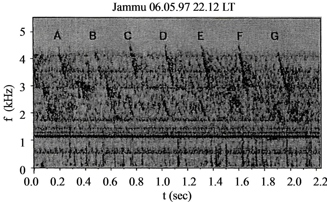
Figure 1(a) presents dynamic spectrum of short whistlers (marked A, B, C, D, E, F and G, selected for the analysis) in the frequency band 3 - 4.5 KHz recorded at Jammu at 2212 IST on June 5, 1997. In the frequency band 1.7 - 3 KHz large number of frequency components are missing and signals resemble more like emissions rather than whistlers. Further, VLF waves in both the frequency bands do not appear simultaneously, rather they appear alternately. Figure 1(b) shows dynamic spectrums of short whistlers (marked 1, 2, 3 and 4, selected for the analysis) and VLF emissions recorded at Jammu at 2147 IST. Whistlers are banded and diffused in the frequency range 2.7 - 3.7 KHz and are repeated in time. The time interval between the events is not con-
 (a)
(a)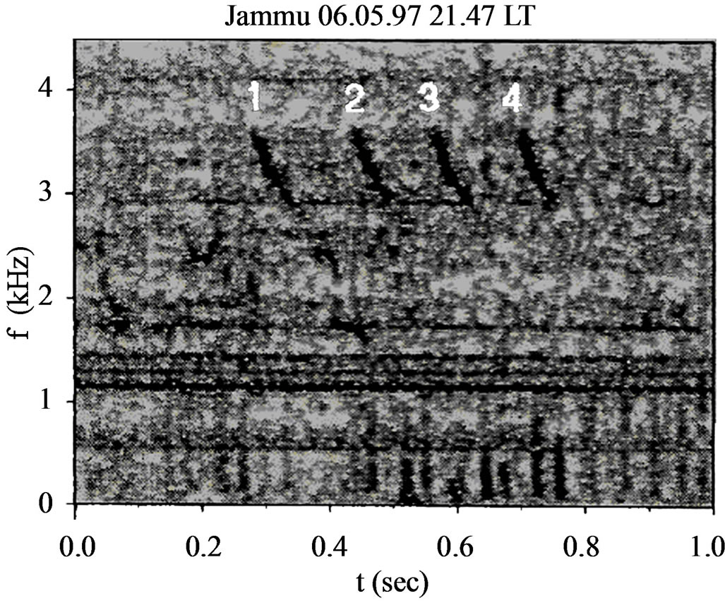 (b)
(b)
Figure 1. (a) Dynamic spectrum of whistlers recorded at Jammu June 5, 1997. Whistlers are marked by A, B, C, D, E, F and G. (b) Dynamic spectrum of whistlers recorded at Jammu June 5, 1997. Whistlers are marked by 1, 2, 3 and 4.
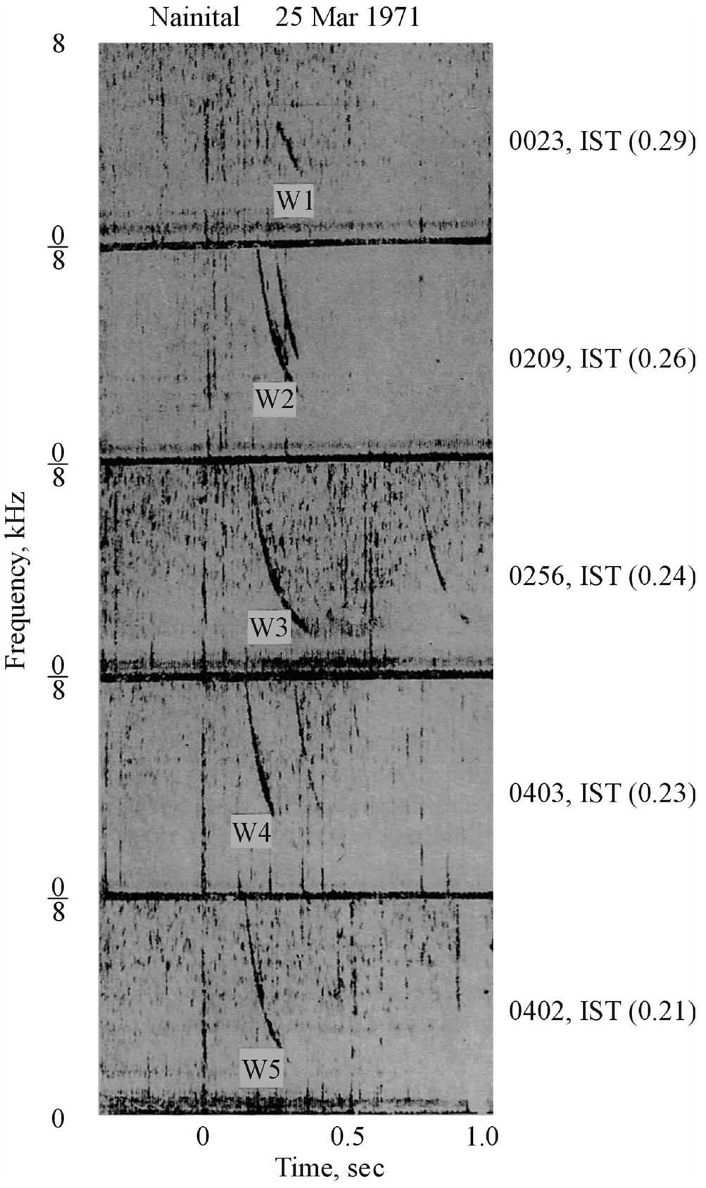
Figure 2. Dynamic spectrum of whistlers recorded at Nainital March 25, 1971. Whistlers are marked by W1, W2, W3, W4 and W5.
stant. Unusual VLF noises are also seen in the spectrum. Figure 2 shows dynamic spectrum of short whistlers selected for the analysis recorded at Nainital on March 25, 1971. The sonograms of sample whistlers (marked W1, W2, W3, W4 and W5) are arranged in a sequence for different time of arrival. Figures 3(a) and (b) shows the dynamic spectra of short whistlers (selected for analysis) recorded at Varanasi on 19 February 1997 at 0017 IST and 2338 IST respectively.
Tarcsai [19] has developed a curve fitting technique for the analysis of middle and high latitude whistlers. This technique has also been applied successfully to those low latitude whistlers whose propagation path are low below L = 1.4 [28-31]. Further technique is found suitable not only for long and good quality whistlers but also for short and faint whistlers. The computer programme written for the purpose requires input data such as frequency time (f, t) values scaled at several points along whistler trace appropriate for F2, zero frequency dispersion (Do), and a suitable ionospheric model etc. The output results include the L-value of propagation, equatorial electron density, total tube content etc. we
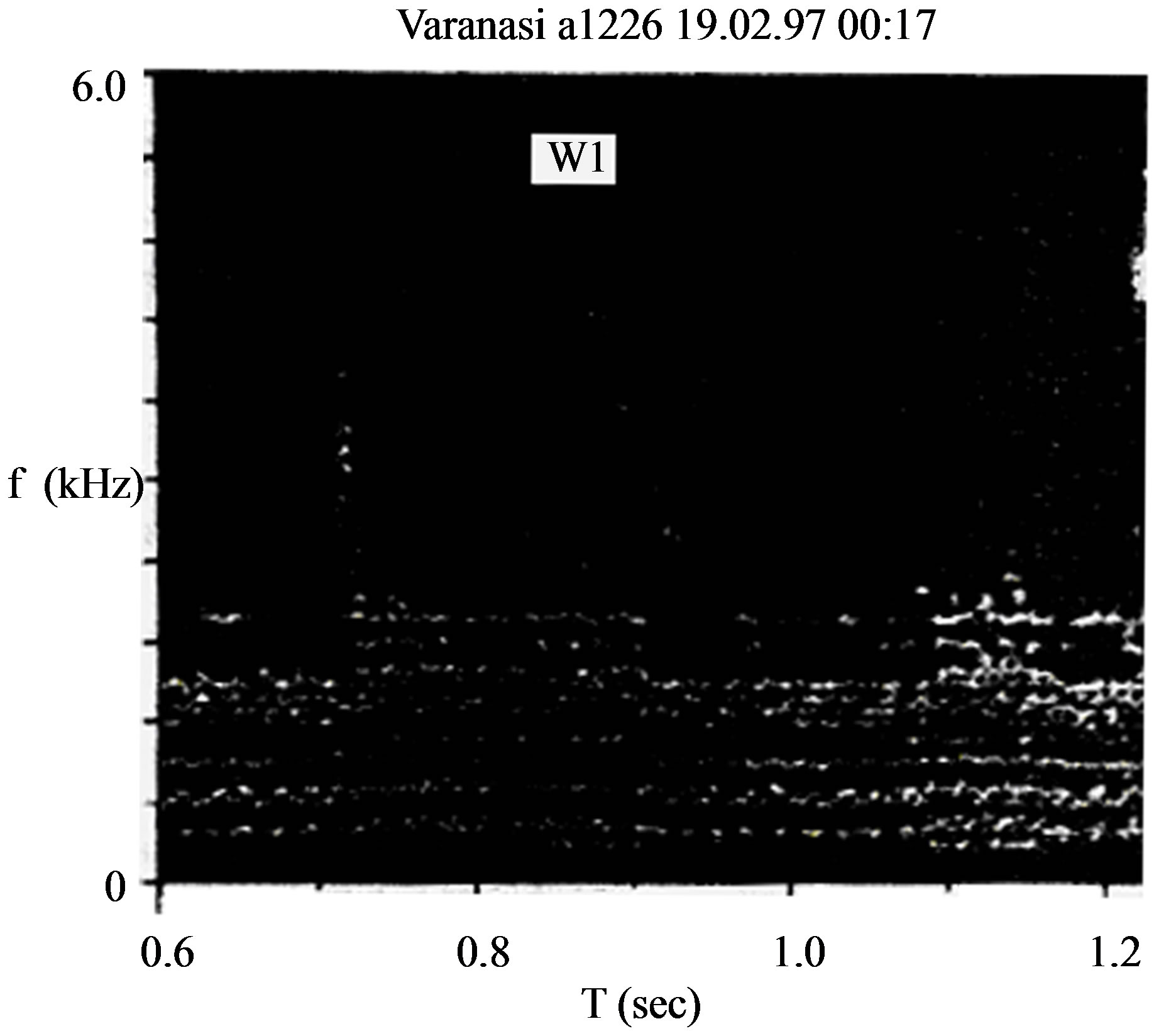
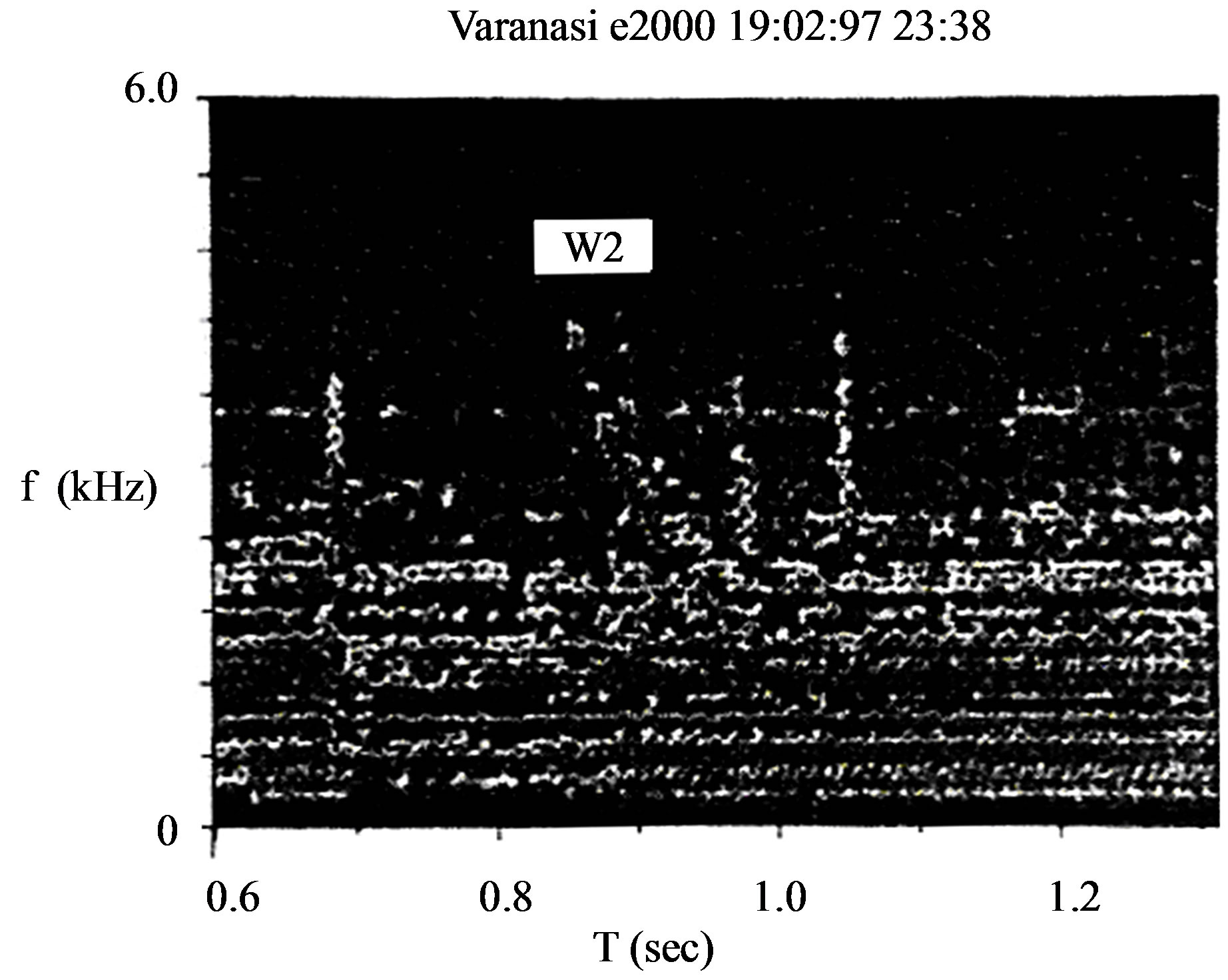
Figure 3. Dynamic spectra of whistlers recorded at Varanasi February 19, 1997. Whistlers are marked by W1 and W2.
have adopted this programme for the analysis of nighttime whistlers recorded at our station Nanital, Varanasi and Jammu during quiet days.
At low L-values, the curve fitting method of Tarcsai [19] would not change too much the equatorial electron density and total electron content values compared to the systematic errors which are inherent in all of the existing nose extension methods. These systematic errors originate from the approximations used for the refractive index and for the ray path in the derivation of the analytic expressions for the dispersion and from the difference between the theoretical and actual distribution plasma along the field lines [32]. To examine its validity we analyzed few whistlers recorded at Jammu using this method as Dowden Allcock [31] Q-technique. Both methods yielded results within ±10%. Further, it is to be noted that the Tarcsai’s method has successfully been used in the analysis of low latitude whistler).
For the determination of Do, fn and tn approximate function for the dispersion of whistlers is given by [19]
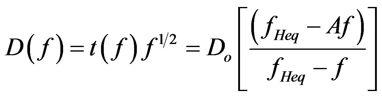 (1)
(1)
where Do = zero frequency dispersion fHeq = equatorial electron gyrofrequency f = Wave frequency
 = travel time at frequency f, and
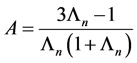 (2)
(2)
Here
where fn is the nose frequency for which travel time tn is written as
 (3)
(3)
If the causative sferic is unknown, and the travel times at different frequencies of the whistler traces are measured with respect to an arbitrary time origin, then it is necessary to introduce a new parameter T, which gives the difference in time between the chosen origin and the actual causative sferic. Using T and Equation (1) the measured travel time  can be written as
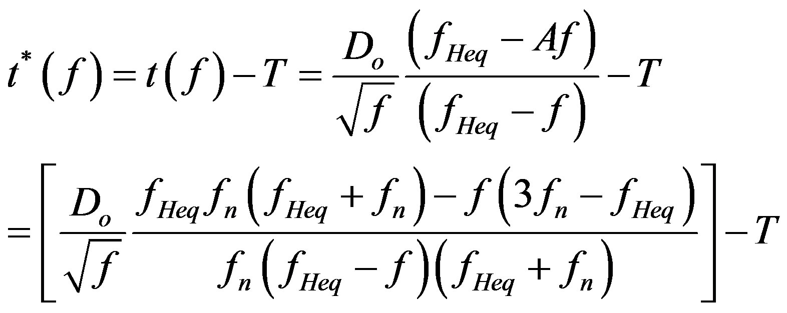 (4)
(4)
In this equation there are four unknown parameters Do, fHe, T and fn. Tarcsai [19] has developed a computer program to solve Equation (4) for the unknown using successive iteration method. In this method those values of Do, fHe, T and fn are searched which give best fit to the measured parameters. After Park (1972) and using Equation (3) for tn.
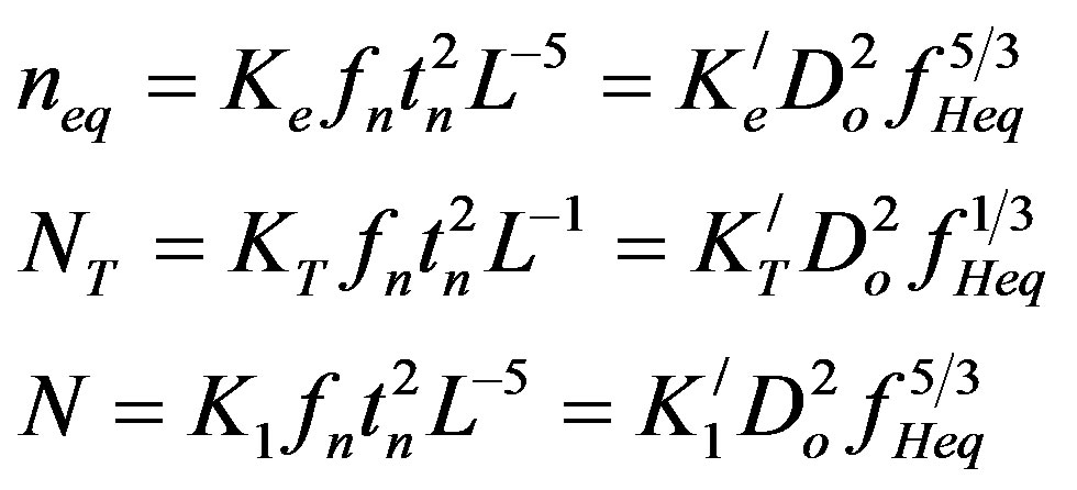 (5)
(5)
Where the constants K/e and K/T are weakly dependent on fn and Λn Tracsai [19].
Using Equation (5) and analyzing whistlers shown in Figures 1-3 recorded at Jammu, Nainital and Varanasi, nose frequency fn, equatorial electron density neq and total electron content NT in a flux tube of unit cross section has been evaluated. Then the equatorial electron temperature Teq was estimated from nose frequency computed from Tarcsai [19] method for a given model of electron distribution for our analysis. A diffusive equilibrium model similar to that adopted by [5,18,19,27], was employed which was represented at the height 1000 km by an electron density 103 electron/cm3, O+ = 90%, H+ = 8%, and He+ = 2% at the temperature  of 1000˚K. The electron temperature in the magnetosphere (Te) is related to the electron temperature at the reference level
  by the equation.
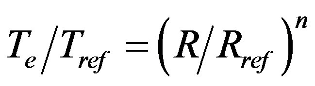 (6)
(6)
where R and Rref are the corresponding geocentric distances. We took two values of n, (n = 1 and 2). For the case of n = 0, Te remains almost constant and for the case of n = 2, Te increases rapidly with height, one expect the actual value of n to lie between these two extremes. The results of the calculation of fn, fHe, Do, L, neq and Teq for the whistlers under consideration are shown in Table 1" target="_self"> Table 1 (for n = 1 and 2).
The whistler nose frequency fn is related to its path L by the approximate relation
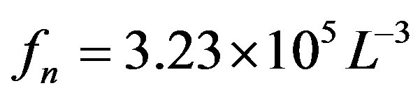 (7)
(7)
Where fn is in kHz and a central dipole magnetic field is used to represent the geomagnetic field. The nose frequency and the minimum equatorial gyrofrequency along the path of propagation are related as [33]
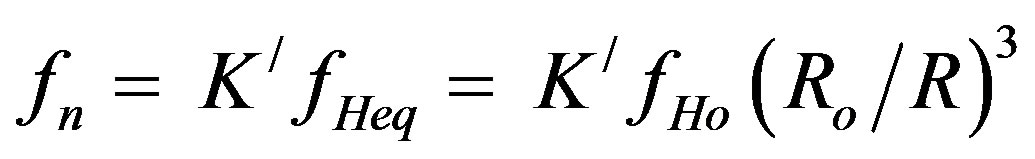 (8)
(8)
Where K/ = 0.38 for a diffusive equilibrium model of the field-line distribution of ionization, fHeq and fHo are the equatorial gyrofrequencies at geocentric distances of R and Ro (Earth’s surface) respectively.
In the equatorial plane the convection electric field, defines as positive in the eastward direction, is given by
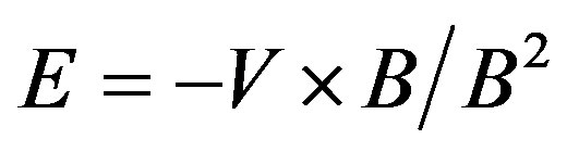 (9)
(9)
In the case of magnetic equator we obtain from Equation (8)
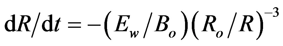 (10)
(10)
where Bo represents the geomagnetic field strength at the
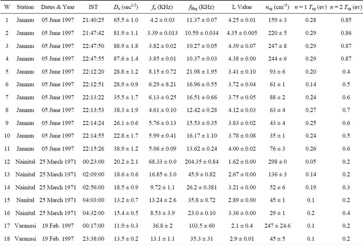
Table 1. Parameters of whistlers observed at Jammu, Naitinal and Varanasi ground stations estimated from the whistler dispersion analysis using accurate curve fitting technique. W is the whistler number, IST is the Indian Standard Time, Do is the dispersion of whistler, fn is the whistler nose frequency, fHeq is equatorial gyro frequency , L-value is in earths radii, neq is the equatorial electron density and Teq is equatorial electron temperature.
Earth’s surface and Ew is the westward component of the magnetospheric electric field. With the help of Equations (7) and (8) the convection electric field in a dipole model in the equatorial plane can be obtained as [34]
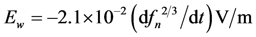 (11)
(11)
With the nose frequency expressed in hartz one can directly estimate the convection electric field from the slope of  using Equation (10). The variation of
  with time for the whistlers observed at Jammu, Nanital and Varanasi are given in Figures 4-6 respectively.
3. Results and Discussion
Several attempts have been made to use whistlers as a diagnostic of the electron temperature of the magnetosphere besides the traditional methods of diagnostics of electron temperature in the magnetosphere. The first such attempt was probably made by Scarf [35] who estimated this temperature from the thermal attenuation of nose whistlers at the upper cut-off frequency. This method was developed by Liemhon and Scarf [36,37], but, to
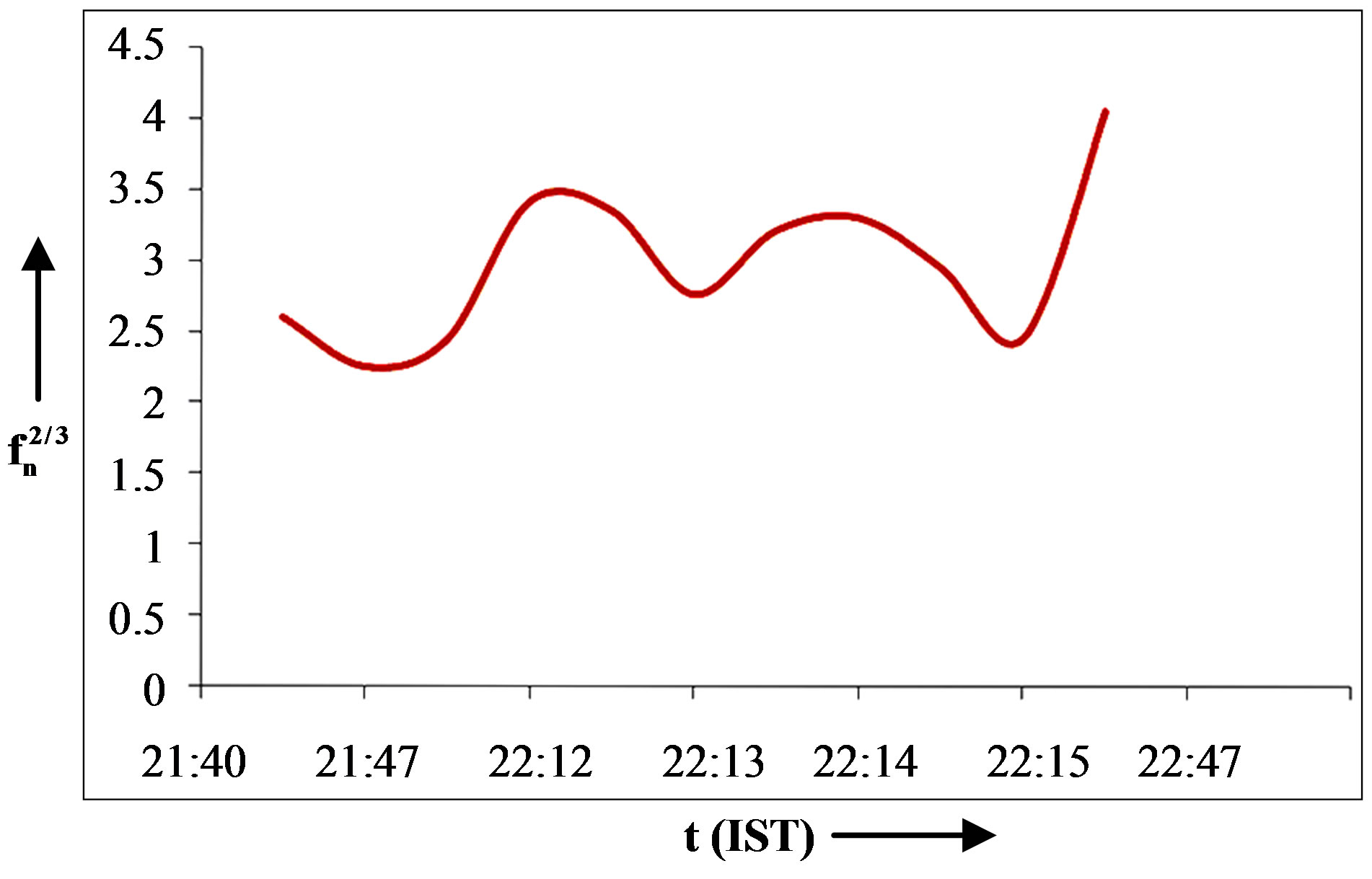
Figure 4. Plot between 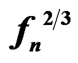 and t for the case observed at Jammu on 05 June 1997.
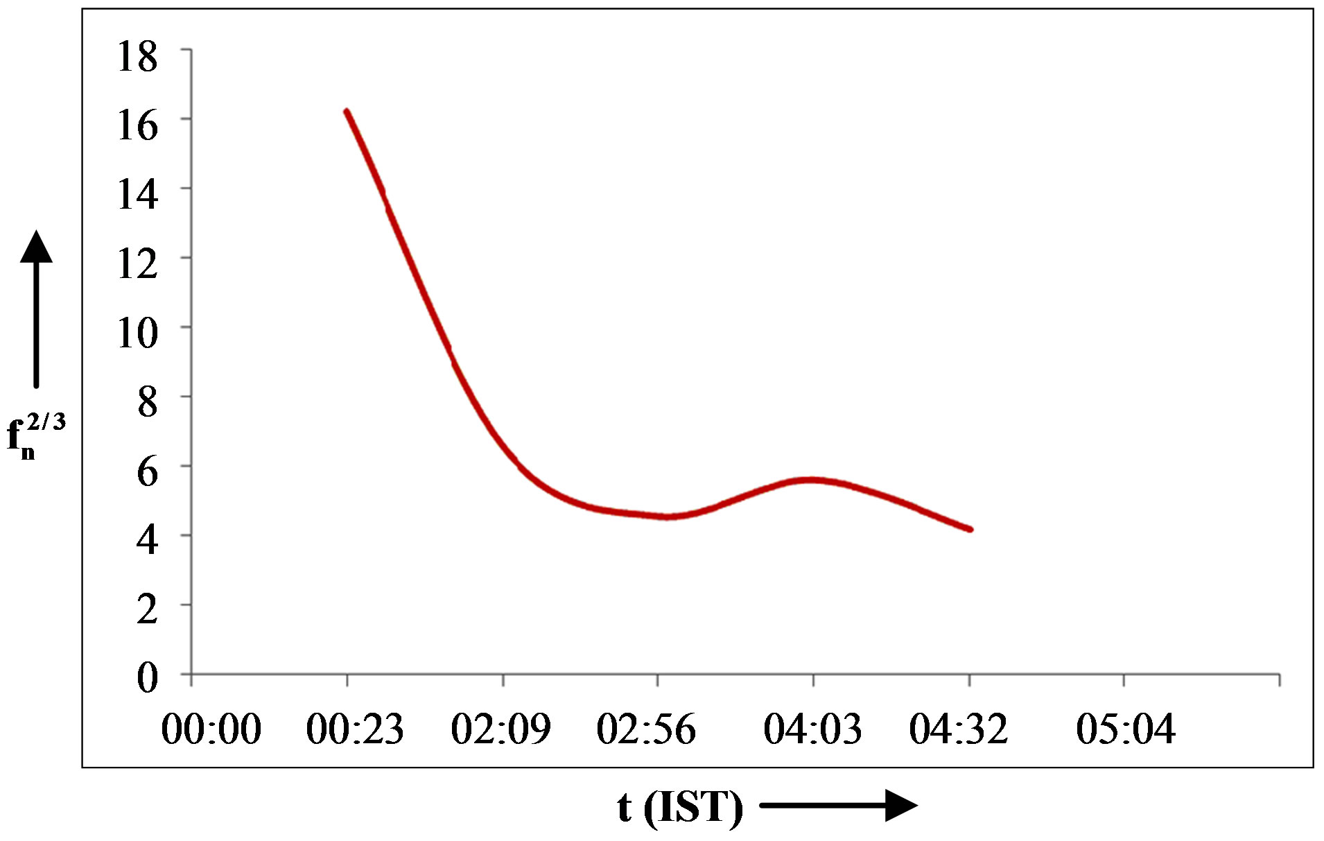
Figure 5. Plot between  and t for the case observed at Nanital on 25 March 1971.
Figure 6. Plot between  and t for the case observed at Varanasi on 19 Feb. 1997.
our knowledge, was never used in practice, perhaps for two reasons. Firstly, it is difficult to decide whether the whistler upper cut-off frequency is determined by wave attenuation or by propagation effects. Secondly, the interpretation of the whistler cut-off frequency in Scarf’s method is very sensitive to the anisotropy of the electron distribution function, which can in general, be determined only by in-situ measurements.
In an alternative approach to this problem, Mc Chesney and Hughes [34] measured the electron density at the magnetospheric equator (neq) by whistler dispersion analysis, and in the topside ionosphere from in situ observations of LHR noise. The ratio of these densities was fitted to a diffusive equilibrium model of electron density distribution with temperature as a parameter. The main assumption was that the electron temperature did not change along the magnetospheric magnetic field line. However, this assumption seems to be incompatible with satellite measurements of electron temperature, equatorial temperatures can be up to a factor of 10 larger than those at ionospheric altitudes [38,39] and needs to be abandoned in further modifications of this method.
A different approach was taken by Guthart [40] who attempted to estimate magnetospheric electron temperature from its effect on whistler group velocity, assuming a gyrofrequency model electron distribution. He predicted that the thermal effect on whistler spectra should be largest at frequencies near the upper cut-off frequency of nose whistlers. However, the size of the effect was less than the experimental error associated with whistler spectral analysis. This conclusion enabled Guthart to estimate an upper bound on the magnetospheric electron temperature of 2 × 10⁴ K ≈ 1.7 eV. By contrast, Kobelev and Sazhin [41] have argued that thermal effects in the vicinity of the plasmapause can be estimated by comparison of observed and theoretical whistler dispersion curves. Assuming an electron density distribution along field lines, they obtained values of electron temperature in the range 7 - 19 eV, depending on the value of the parameter n. This temperature corresponds to an average temperature of all electrons “cold” ones with energies ≤ 1 eV plus small “hot” components with energies of the order 1 keV. In both these papers the effect of variation of the electron temperature along the magnetospheric magnetic field line was neglected as was done by Mc Chesney and Hughes [34]. More accurate analysis by Sazhin et al. [42], based on the DE-1, 2, 3, 4 models described earlier, let to a result rather close to that of Guthart [40], namely, the magnetospheric electron temperature was estimated to be blow 4 eV and depends on the choice of electron distribution model.
Sazhin et al. [43] discussed different approaches to this type of diagnostic technique and have concluded that the most effective way to estimate the electron temperature with the help of ground—observed whistlers would be to use nose whistlers with the well-defined upper branch and compare whistler group delay times at the nose and at the upper cut-off frequency. Recently, Sazhin et al. [44] have extended this approach of analysis to a larger number of whistlers in order to get statistically more significant results. They have shown that the estimated magnetospheric electron temperature strongly depends on the choice of model of electron distribution along the magnetospheric magnetic field line.
The whistler data recorded at Jammu, Nainital and Varanasi at different times and for different magnetic activities have been analysised to estimate the magnetospheric electron temperature in the vicinity of magnetospheric equator at low latitudes. We have applied the curve-fitting technique of Tarcsai [19] for our non-nose whistlers at these stations to derive the magnetospheric electron temperatures. The estimated temperature of magnetospheric electrons inferred from the whistler data shown in Table 1 is about 0.8 eV for the value of n = 2 and is about 0.25 eV for the value of n = 1. Our mean value of Teq obtained using the diffusive equilibrium model estimated by the method of curve-fitting technique of Tarcsai [19] is ~0.5 eV, slightly smaller with other estimates of electron temperature in the equatorial plasmasphere (see Guthart, 1965, 1973; Sazhin et al., 1993; Sazhin et al., 1990, 1992). Magnetospheric temperatures are quite variable inferred temperatures between 5 × 10³ K and 3 × 10⁴ K; similar electron temperatures were deduced in a more detailed study by Decreau et al. [45] and it would be unwise to attempt to generalize our results.
We have also estimated the above electric field on the basis of dipole geomagnetic field. However, both ground-based and satellite brone magnetometer data shows that fast changes in the magnetic field takes place during substorm commencement and substorm expansion and recovery phase. Wang and Kim (1972) have discussed the decaying ring current and the electric field that may be associated with that decay. Thus, the departure from the dipole field model gives an induced electric field due to temporal changes in the geomagnetic field.
In the present study the magnetospheric electric field in the plasmasphere at different L-values is found to be eastward in the pre-midnight sector and westward in the post-midnight sector, in agreement with the published results [12,13,46]. The magnitude of the eastward electric field is about 0.35 mV/m in the equatorial plane of Jammu. The westward electric field comes out to be about 0.72 mV/m for Nanital and 0.12 mV/m for Varanasi.
Thus the present results of electric field agrees with the results of Ionosonde observations of the night-time F-layer during substorm, and are in good agreement with the results reported by Park [46]. In the Ionosonde studies, it was found that during winters, the F-layer settles down to a quasi steady state. Its response to the magnetospheric substorm activity consists of a large scale distortion with F-layer lifted upward in the pre-midnight sector and pushed downward in the post-midnight sector. This distortion was interpreted as the result of E × B drift by an eastward electric field before midnight and by a westward field after midnight. This reversal in the electric field direction is confirmed by the low latitude whistler results reported here. The reversal of the electric field direction near midnight as shown in Figures 4-6 with the westward component during post-midnight hours and an eastward component during pre-midnight hours was also observed by the barium cloud technique and by electrostatic probes on balloons.
4. Conclusion
The non-nose whistlers recorded at Jammu, Nainital and Varanasi have been analyzed to estimate the equatorial electron density, electron temperature and electric field in the equatorial magnetosphere. The estimated temperature and electric field are slightly smaller compared to the estimated value of other workers. This preliminary test of our method of temperature diagnostic is rather encouraging. However, before this method can be recommended for practical applications, we need to specify the model of electron density, temperature distribution, and electric field in the magnetosphere more accurately, so as to have a better estimate for the effect ducted ray paths and increase the precision of determining whistler parameters. Actually it is the first attempt to estimate the above mentioned parameters by using non-nose whistler data recorded at Jammu, Nainital and Varanasi.
5. Acknowledgements
M. Altaf, M. M. Ahmad and J M Banday are thankful to Director, NIT Srinagar, Kashmir, India for his constant encouragement and support.
REFERENCES
- V. V. Somayajulu and B. A. P. Tantry, “Whistlers at Low Latitudes,” Indian Journal of Radio & Space Physics, Vol. 1, 1972, pp. 102-118.
- P. Chauhan and B. Singh, “High Dispersion Whistlers Observed at Agra Station (L = 1.15),” Planetary and Space Science, Vol. 40, No. 6, 1992, pp. 873-877.
- P. N. Khosa, Lalmani and K. Kishen, “An Analysis of Low Latitude Whistlers Observed at Nainital,” Indian Journal of Physics, Vol. 64B, No. 1, 1990, pp. 34-41.
- C. G. Park, “Methods of Determining Electron Concentration in the Magnetosphere from Nose Whistlers,” Tech. Rep. 3454-I, Stanford University, Stanford, 1972.
- C. G. Park and D. L. Carpenter, “Whistler Observations of the Interchange of Ionization between the Ionosphere and the Protonosphere,” Journal of Geophysical Research, Vol. 75, No. 22, 1970, pp. 4249-4260.
- S. S. Sazhin, M. Hayakawa and K. Bullough, “Whistler Diagnostic of Magnetospheric Parameters: A Review,” Annales Geophysicae, Vol. 10, No. 5, 1992, pp. 193-308.
- R. A. Helliwell, “Whistlers and Related Ionospheric Phenomena,” Stanford University Press, Stanford, 1965.
- C. G. Park, “Some Features of Plasma Disturbation in the Plasma Sphere Deduced from Antartic Whistlers,” Journal of Geophysical Research, Vol. 79, No. 1, 1974, pp. 169-173.
- G. P. Tarcsai, Szemeredy and L. Hegymegi, “Average Electron Density Profiles in the Plasmasphere between L = 1.14 and 3.2 Deduced from Whistlers,” Journal of Atmospheric and Solar-Terrestrial Physics, Vol. 50, 1988. pp. 607-611.
- Lalmani, M. K. Babu, R. Kumar, R. Singh and A. K. Gwal, “An Explanation of Daytime Discrete VLF Emissions Observed at Jammu (L = 1.17) and Determination of Magnetospheric Parameters,” Indian Journal of Physics, Vol. 74B, No. 2, 2000, p. 117.
- D. L. Carpenter and C. G. Park, “On What Ionospheic Workers Should Know about the Plasmapouse and Plasmasphere,” Reviews of Geophysics and Space Physics, Vol. 11, 1973, pp. 133-154.
- M. K. Andrews, “Night Time Radial Plasma Drifts and Coupling Fluxes at L=2.3 from Whistler Mode Measurements,” Planetary and Space Science, Vol. 28, No. 4, 1980, pp. 407-417.
- D. L. Carpenter and R. L. Smith, “Whistler Measurements of Electron Density in the Magnetosphere,” Reviews of Geophysics, Vol. 2, No. 3, 1964, pp. 415-441.
- H. B. Liemohn and F. L. Scarf, “Exospheric Electron Temperatures from Nose Whistler Attenuation,” Journal of Geophysical Research, Vol. 67, No. 5, 1962, pp. 1785- 1789.
- S. S. Sazhin, P. Bognar, A. J. Smith and G. Tarcsai, “Magnetospheric Electron Temperature Inferred from Whistler Dispersion Measurements,” Annales Geophysicae, Vol. 11, 1993, pp. 619-623.
- R. P. Singh, A. K. Singh and D. K. Singh, “Plasmaspheric Parameters as Determined from Whistler Spectrograms: A Review,” Journal of Atmospheric and Solar-Terrestrial Physics, Vol. 60, No. 5, 1998, pp. 494-508.
- B. Singh and H. Hayakawa, “Propagation Mode of Lowand Very-Low-Latitude Whistlers,” Journal of Atmospheric and Solar-Terrestrial Physics, Vol. 63, No. 11, 2001, pp. 1133-1147.
- R. P. Singh, K. Singh, A. K. Singh, D. Hamar and J. Lichenberger, “Matched Filtering Analysis of Diffuded Whistlers and Its Propagation Characteristics at Low Latitudes,” Journal of Atmospheric and Solar-Terrestrial Physics, Vol. 68, 2006, pp. 710-714.
- G. Tarcsai, “Routine Whistler Analysis by Means of Accurate Curve Fitting,” Journal of Atmospheric and Terrestrial Physics, Vol. 37, No. 11, 1975, pp. 1447-1457.
- R. P. Singh, D. K. Singh, A. K. Singh, D. Hamar and J. Lichenberger, “Application of Matched Filtering and Parameter Estimation Technique to Low Latitude Whistlers,” Journal of Atmospheric and Solar-Terrestrial Physics, Vol. 61, No. 14, 1999, pp. 1081-1093.
- D. Hamar, G. Tarcsai, J. Lichtenberger, A. J. Smith and K. H. Yearby, “Fine Structure of Whistlers Recorded Digitally at Hally, Antarctica,” Journal of Atmospheric and Terrestrial Physics, Vol. 52, No. 9, 1990, pp. 801-810.
- D. Hamar, Cs. Ferencz, J. Lichtenberger, G. Tarcsai, A. J. Smith and K. H. Yearby, “Trace Splitting of Whiltlers: A Signature of Fine Structure or Mode Fitting in Magnerospheric Ducts?” Radio Science, Vol. 27, No. 2, 1992, pp. 341-346.
- L. O. Hines, “The Upper Atmosphere in Motion,” Quarterly Journal of the Royal Meteorological Society, Vol. 89, No. 379, 1963, pp. 1-42. http://dx.doi.org/10.1002/qj.49708937902
- K. Maeda and I. Kato, “Electrodynamics of the Ionosphere,” Space Science Reviews, Vol. 5, No. 1, 1966, pp. 57-79. http://dx.doi.org/10.1007/BF00179215
- Lalmani, R. Kumar, R. Singh and B. Singh, “Characteristics of the Observed Low Latitude Very Low Frequency Emission Periods and Whistler Mode Group Delay at Jammu,” Indian Journal of Radio & Space Physics, Vol. 30, 2001, pp. 214-216.
- M. Rao and Lalmani, “An Evaluation of Duct Life Times from Low Latitude Ground Observations of Whiltlers,” Planetary and Space Science, Vol. 23, No. 6, 1975, pp. 923-927.
- R. P. Singh, R. P. Patel, A. K. Singh, D. Hamar and J. Lichenberger, “Matched Filtering and Parameter Estimation Method and Analysis of Whistlers Recorded at Varanasi,” Pramana, Vol. 55, No. 5-6, 2000, pp. 685-691.
- M. J. Rycroft and A. Mathur, “The Determination of the Minimum Group Delay of a Non-Nose Whistlers,” Journal of Atmospheric and Terrestrial Physics, Vol. 35, No. 12, 1997, pp. 2177-2182.
- D. Ho and L. C. Bernard, “A Fast Method to Determine the Nose Frequency and Minimum Group Delay of Whistlers When the Causative Spheric Is Unknown,” Journal of Atmospheric and Terrestrial Physics, Vol. 35, No. 5, 1973, pp. 881-887.
- M. Hayakawa, Y. Tanaka, S. S. Sazhin, M. Tixiier and T. Okada, “Substorm-Associated VLF Emissions with Frequency Drift in the Premidnight Sector,” Journal of Geophysical Research, Vol. 93, 1988, pp. 5685-5700.
- R. L. Dowden and G. Mck Allcock, “Determination of Nose Frequency of Non-Nose Whistlers,” Journal of Atmospheric and Terrestrial Physics, Vol. 33, No. 7, 1971, pp. 1125-1129.
- G. Tarcsai, Candidate of Science Thesis, Hungarian Academy of Sciences, Budapest, 1981.
- J. J. Angerami, “Whistler Study of the Distribution of Thermal Electrons in the Magnetosphere,” Stanford University, Stanford, 1966.
- J. Mc Chesney and A. R. D. Hughes, “Temperature in the Plasmasphere Determined from VLF Observations,” Journal of Atmospheric and Terrestrial Physics, Vol. 45, No. 1, 1983, pp. 33-39.
- F. L. Scarf, “Landau Damping and the Attenuation of Whistlers,” Physics of Fluids, Vol. 5, No. 1, 1962, pp. 6- 13.
- H. B. Liemohn and F. L. Scarf, “Whistler Attenuation by Electron with an E−2.5 Distribution,” Journal of Geophysical Research, Vol. 67, No. 11, 1962, pp. 4163-4167.
- H. B. Liemohn and F. L. Scarf, “Whistler Determination of Electron Energy and Density Distribution in the Magnetosphere,” Journal of Geophysical Research, Vol. 69, No. 5, 1964, pp. 883-904.
- G. P. Serbu and E. J. R. Maier, “Low Energy Electrons Measured on IMP2,” Journal of Geophysical Research, Vol. 71, No. 15, 1966, pp. 3755-3766.
- Seely, “Whistler Propagation in a Distorted Quiet Time Model Magnetosphere N.T,” Tech. Rep. 3421-I, Stanford University, Stanford, 1977.
- H. Guthart, “Nose Whistler Dispersion as a Measure of Magnetospheric Electron Temperature,” Radio Science, Vol. 69D, 1965, pp. 1417-1424.
- V. V. Kobelev and S. S. Sazhin, “An Estimate of Magnetospheric Electron Temperature from the Whistler Spectrograms,” Journal of Technical Physics (Letters), Vol. 9, 1983, pp. 862-865.
- S. S. Sazhin, A. J. Smith and E. M. Sazhin, “Can Magnetospheric Electron Temperature Be Inferred from Whistler Dispersion Measurements,” Annales Geophysicae, Vol. 8, 1990, pp. 273-285.
- S. S. Sazhin, M. Hayakawa and K. Bullough, “Whistler Diagnostic of Magnetospheric Parameters: A Review,” Annales Geophysicae, Vol. 10, No. 5, 1992, pp. 293-308.
- S. S. Sazhin, P. Bognar, A. J. Smith and G. Tarcsai, “Magnetospheric Electron Temperatures Inferred from Whistler Dispersion Measurements,” Annales Geophysicae, Vol. 11, 1993, pp. 619-623.
- P. M. Decreau, C. Beghin and M. Parrot, “Global Characteristics of the Cold Plasma in the Equatorial Plasmapause Region as Deduced from the GEOS-I Mutual Impedance Probe,” Journal of Geophysical Research, Vol. 87, 1982, pp. 695-712.
- C. G. Park, D. L. Carpenter and D. B. Wiggin, “Electron Density in the Plasmasphere: Whistler Data on Solar Cycle Annual and Diurnal Variations,” Journal of Geophysical Research, Vol. 83, No. A7, 1978, pp. 3137-3144.