International Journal of Geosciences
Vol.5 No.2(2014), Article ID:43200,12 pages DOI:10.4236/ijg.2014.52020
Estimation of the Effect of Anisotropy on Young’s Moduli and Poisson’s Ratios of Sedimentary Rocks Using Core Samples in Western and Central Part of Tripura, India
Jwngsar Brahma, Anirbid SircarPandit Deendayal Petroleum University, Gandhinagar Raisan Village, Raisan, India
Email: jwngsar.brahma@spt.pdpu.ac.in
Copyright © 2014 Jwngsar Brahma, Anirbid Sircar. This is an open access article distributed under the Creative Commons Attribution License, which permits unrestricted use, distribution, and reproduction in any medium, provided the original work is properly cited. In accordance of the Creative Commons Attribution License all Copyrights © 2014 are reserved for SCIRP and the owner of the intellectual property Jwngsar Brahma, Anirbid Sircar. All Copyright © 2014 are guarded by law and by SCIRP as a guardian.
Received December 22, 2013; revised January 19, 2014; accepted February 16, 2014
Keywords:Elastic Stiffness; Shales; Sandstone; Sedimentary Rock; Anisotropy
ABSTRACT
The velocity anisotropy parameters and elastic constants play a very important role to estimate Young’s modulus and Poisson’s ratios accurately. For geomechanics applications such as hydraulic fracturing design, analysis of wellbore stability and rock failure, determination of in situ stress and assessment of the response of reservoirs and surrounding rocks to changes in pore pressure and stress, Young’s modulus and Poisson’s ratios play a very important role. Four rock samples were collected from four different wells situated in study area. The ultrasonic transmission method has been used to measure P-wave, Sh-wave and Sv-wave travel times as a function of orientation and confining pressure. The five independent stiffnesses constants, Young’s moduli, Poisson’s ratios and Bulk moduli of the samples were estimated. The Poisson’s ratios ( and
and ) are varying as the confining pressure is changed. The axial strain is larger than the lateral strain, resulting
  wang##Bracket#. For shales, the Young’s modulus measured parallel to bedding E1 is usually greater than the Young’s modulus measured perpendicular to bedding E3. Through this study it has been observed that, there is a strong effect of anisotropy parameters on Young’s modulus and Poisson’s ratio.
1. Introduction
In hydrocarbon exploration and production theory, one of the common assumptions in conventional seismic exploration is the subsurface consisting of a series of elastically homogenous isotropic layers. That assumption is not true; numerous investigations during the previous decades have demonstrated the presence of seismic anisotropy in different geological settings and on various scales [1]. Ignoring these anisotropy effects can adversely influence the result of most basic seismic data processing and interpretation steps, such as NMO correction, velocity analysis, stacking, migration, DMO correction, time to depth conversion and AVO analysis [1-4].
The earth material is said to be transversely isotropic with vertical axis of symmetry if the elastic properties vary vertically but not horizontally in the simplest horizontal or layered case. Detecting and quantifying this type of anisotropy are very useful for correlation of sonic logs in vertical and deviated wells and for borehole surface seismic imaging and studies of amplitude variation with offset (AVO). The yield information about rock stress and fracture density and orientation can be estimated by identifying and quantifying the elastic anisotropy and these parameters are useful for designing hydraulic fracture jobs and for understanding horizontal and vertical permeability anisotropy. To understand the elastic anisotropy for more complex cases, such as dipping layers, fractured layered rocks or rocks with multiple fracture sets, superposition of the effects of the individual anisotropies is necessary.
In spite of the fact that shale formations exhibit high anisotropies, the study of fracture related anisotropy has been more intensive, both theoretically [5-12] and experimentally [13-15]. This is most likely explained because when anisotropy is observed it can be associated with fractures, which have a strong impact on permeability. Highly permeable rocks can be a good oil reservoir. However, in order to associate anisotropy with fracture zone, a correction for the anisotropic effect of the upper layers of the sedimentary column that is traversed by the wave field is necessary. More recently, the influence of pore fluid on elastic properties of shale has been investigated. Hornby measured compressional and shear wave velocities up to 80 MPa on two fluid saturated shale samples under drained conditions [16]. One sample from Jurassic outcrop shale was recovered from under sea and stored in its natural fluid, and the other is Kimmeridge clay taken from a North Sea borehole. Measurements were made on cores parallel, perpendicular, and at 45˚ to bedding. Values of anisotropy were up to 26% for compressional and 48% for shear wave velocity, and were found to decrease with increasing pressure. The effect of reduced porosity was, therefore, concluded to be more influential on anisotropy than increased alignment of minerals at higher pressure. The elastic constants, velocities and anisotropies in shales can be obtained from traditionally measured on multiple adjacent core plugs with different orientations [17]. To derive the five independent constants for transversely isotropic (TI) rock, Wang measured three plugs separately (one parallel, one perpendicular, and one  to the symmetric axis). The advantage of this three plugs method is redundancy for calculation of the five independent elastic constants, since each core plug measurement yields three velocities.
Sandstones are rarely clean; they often contain minerals other than quartz, such as clay minerals, which can affect their reservoir qualities as well as their elastic properties. The presence of clay mineral and clastic sheet silicates strongly influences the physical and chemical properties of both sandstones and shales [18]. Clay can be located between the grain contacts as structural clay, in the pore space as dispersed clay, or as laminations [19]. The distribution of the clay will depend on the conditions at deposition, on compaction, bioturbation and diagenesis. While most reservoirs are composed of relatively isotropic sandstones or carbonates, their properties may be modified by stress. Non-uniform compressive stress will have a major effect on randomly distributed microcracks in a reservoir. When the rock is unstressed all of the cracks may be open, however, compressional stresses will close cracks oriented perpendicular to the direction of maximum compressive stress, while cracks parallel to the stress direction will remain open. Elastic waves passing through the stressed rock will travel faster across the closed cracks (parallel to maximum stress) than across the open ones. The sands and sandstone are intrinsically isotropic unless they are fractured, finely layered or clay bearing. Wang shows that the brine-saturated Africa reservoir sands, which are essentially clay free, have very little anisotropy (average P-anisotropy and Sanisotropy are probably within the measurement uncertainties) [17]. For the brine saturated tight sands, the anisotropy is 5.0% for the P-wave and 3.3% for the S-wave when averaged over all samples at all pressures. At the net reservoir pressure of 7500 psi (51.7 MPa), anisotropy is slightly lower, averaging 4.6% and 3.2% for P-and S-waves, respectively. Gas-saturated tight sands and shaly sands show some degrees of anisotropy, ranging from 0% to 36% for P-waves and 0.3% to 19.5% for S-waves. When averaged at all pressures, the anisotropy is 9.9% for the P-wave and 5.5% for the S-wave.
There are various methods to estimate anisotropy parameters. Wang presented a method for measuring seismic velocities and transverse isotropy in rocks using a sing core plug [17]. Wang pointed out that shale cores must be preserved. Otherwise, once a shale core is dehydrated, fractures will develop along the bedding plane, and the measured seismic velocities and anisotropy will no longer be accurate [20].
Leslie [21] determined the Thomsen anisotropic parameters ε and δ by measurement of head wave velocities along the seismic lines. This method obtained more realistic anisotropic parameters than those measured in the laboratory, but needs to ensure that the spread is of sufficient length so that the refractor velocities measured are from rocks below the weathered layer.
In this paper four kinds of core samples; Dry Sandstone, Shale, Sandy Shale and Saturated Sandstone were collected from Tripura oil field. The purpose of this paper is to estimate effects of elastic anisotropic on Young’s moduli and Poison’s ratios. We used the ultrasonic transmission method to measure Vp, Vsh and Vsv wave velocities, as function of confining pressure from 1 MPa to 40.3 MPa. Using these velocities five independent stiffnesses have been calculated and hence Thomsen’s parameters as well as geo-mechanical parameters.
2. Methodology
2.1. Sample Preparation
The four kinds of core samples namely dry sandstone, shale, sandy shale and saturated sandstone were collected from the Tripura field in the zone between 1910 - 2200 m and were analysed. Each specimen had diameter 25.4 mm and length 50 mm. The samples had significant lattice preferred orientation. Before performing the test the specimens were cored using diamond drill and the ends of the specimens were ground flat and parallel to  To get more effective result the samples were also checked for flaws and defects. In a vacuum oven at 170˚C for 20 hours the specimens were dried. Next, using digital balance the dry mass of samples was measured. The dry bulk density was computed by dividing the volume by the mass of the samples. After completing, the sandstone was water saturated and the bulk density was computed.
2.2. Experiment Procedure
For each specimens three velocities were measured, one compressional wave and two orthogonal shear wave as a function of pore pressure and confining pressure. Each specimen was jacketed and secured between a matched set of ultrasonic transducers having resonant frequency 1.0 MH. Specimen reference system has the x-axis parallel to the lamination in the foliation, the y-axis normal to the lineation in the foliation and z-axis perpendicular to the foliation plane. Main frequency of ultrasound transducer is 1 MHz. Volume change can obtained from linear strains in three directions which is determined from the piston displacement through necessary correction. Each polarization is sequentially propagated through the rock and each waveform is determined from the data using the appropriate correction for the travel time through the transducer assembly. The experiments, on dry and saturated specimens, were conducted at confining pressures from 1 Mpa to 40.3 Mpa.
It is necessary to core specimens in three directions: vertical, horizontal and at an intermediate angle between vertical and the plane of isotropy (Figure 1), to measure traverse isotropy completely. Three velocities were measured in each direction, leading total nine velocities

Figure 1. Traditional three-plug method for measuring transverse isotropy in laboratory core samples. Three adjacent core plugs (one parallel, one perpendicular, and one ±45 to symmetry axis) must be cut from whole cores and velocities measured to derive the five elastic constants (Wang, 2002).
for each sample. The particle polarization and the direction of propagation of the three modes of propagation, P Sh and Sv in the stratigraphic column within the zone of interest are shown in Figure 2.
Both in room dry and full water saturation conditions, sandstone specimens were tested. But for shale and sandy shale it is difficult in saturating these rocks. So, only in room dry conditions the shale and sandy shale specimens were tested.
It was assumed that, the effective hydrostatic pressure is the difference between confining pressure and pore pressure. The pore pressure was kept constant while the confining pressure varied (drained regime). The confining pressure was varied from atmospheric pressure up to the reservoir effective pressure condition in dry specimen. But the effective pressure never exceeded the reservoir pressure in saturated specimens. However the pore pressure was varied from atmospheric pressure up to a pressure approximately 32% higher than the reservoir pressure condition.
2.3. Mathematical Analysis
In this paper only the standard three plug method will be discussed since it is commonly used in oil exploration. Standard three plug method is by far the most common measurement approach. The method requires the extraction of three core plug along prescribed orientation relative to the assumed symmetric axes. These orientations are parallel, perpendicular and typically 45˚ to the vertical symmetry axis. Either static or dynamic ultrasonic laboratory measurements can be performed on these plugs to provide the magnitude of tensor elements  and
and  (Mavko, 1986). These five elastic constants can be recast into more geophysical meaningful parameter [1].
The relation between stress  and strain
  in vertical transverse isotropy (VTI) is given by the following relation as:
 (1)
(1)
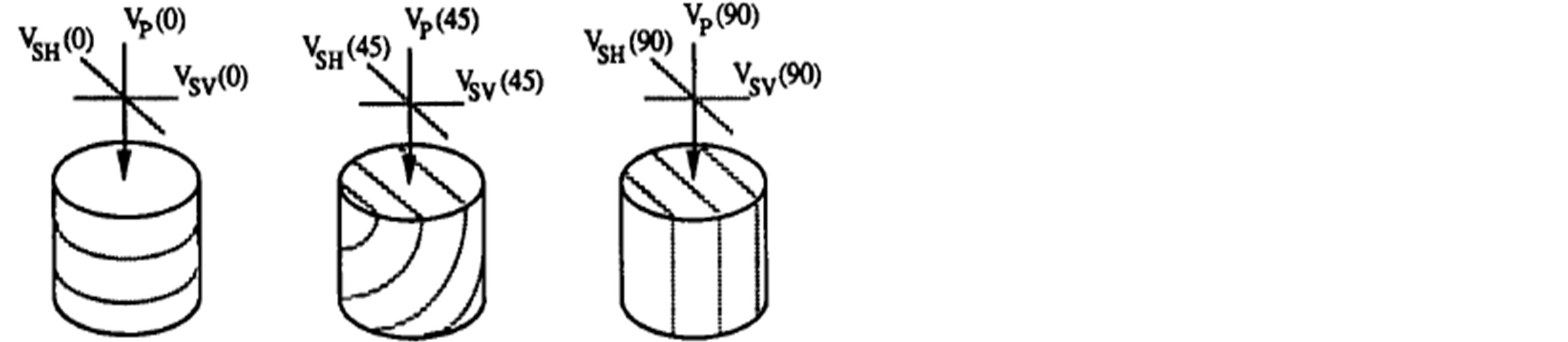
Figure 2. Scheme of sample preparation and velocity measurements in shales. Wave propagation and polarization with respect to bedding-parallel lamination is shown. Numbers in parentheses indicate the phase velocity angle with respect to the bedding-normal symmetry axis (Vernik and Nur, 1992).
where Cijkl is the Voigt matrix [22].
From Figure 1 it is seen that if the axis is denoted by Z, the other two principal axes (X and Y) are parallel to the transversely isotropic plane. In this coordinate system, the stiffness matrix C is expressed as:
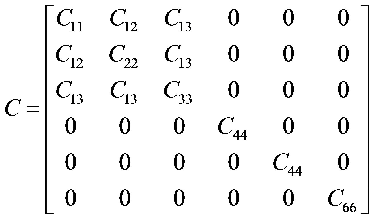 (2)
(2)
From the above Equation (2), Voigt matrix C, there are five non-zero independent elastic constants: 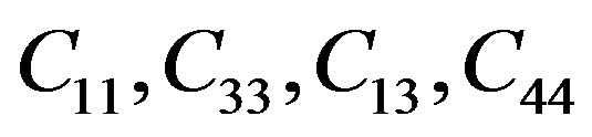 and
and . The sixth elastic constant is
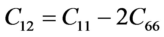 . Here,
  is the in-plane compressional modulus,
  is the out-of-plane compressional modulus,
  is the out-of-plane shear modulus, and
  is the in-plane shear modulus,
  is an important constant that controls the shape of the wave surfaces.
Using five elastic stiffness Cij , a bulk modulus, one vertical Young’s moduli, E3 and one horizontal Young’s modulus E1 and three dynamic Poisson’s ratios can be determines for a hexagonal material as follows [23]:
 (3)
(3)
 (4)
(4)
 (5)
(5)
 (6)
(6)
 (7)
(7)
 (8)
(8)
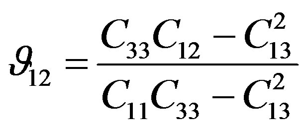
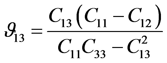
These dynamic Poison’s ratios Equations (7) and (8),  , are indirect measure of the ratio of the lateral to axial strains when the uniaxial stress is applied in the same direction of axial strain.
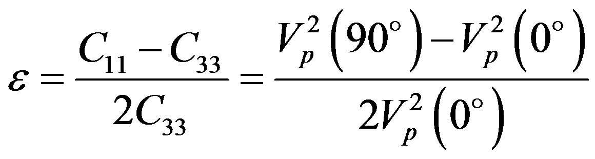
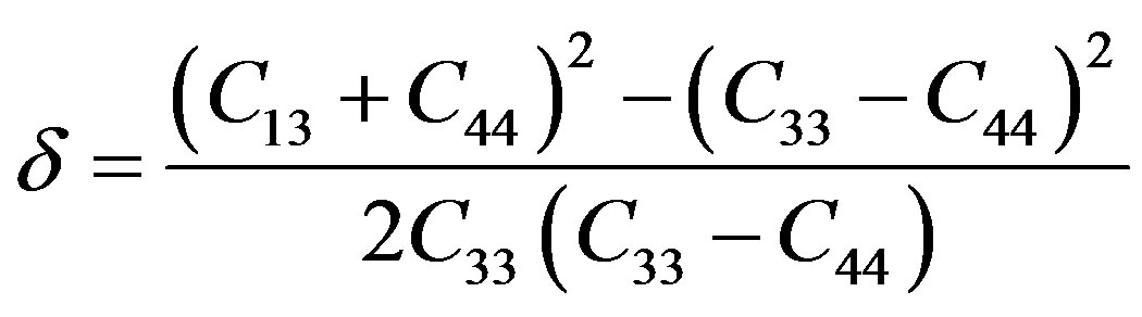
There are three types of velocity anisotropies ( and
and ) known as Thomsen’s parameters and can be estimated by the following mathematical equations suggested by Thomsen [1]:
 (9)
(9)
 (10)
(10)
 (11)
(11)
3. Result and Discussion
Four types of rock samples that represent elastic and anisotropy behaviour in the sedimentary column: dry sandstone, saturated sandstone, shale and sandy shale have been collected from Tripura oil filed. Each of these rocks types exhibit varying sensitivities to confining pressure, and as a consequence the anisotropies are affected differently as the confining pressure varies. The behaviour of the elastic anisotropy for the different rock types as the confining pressure is increased (Figures 3-6).

Figure 3. Comparison of Thomsen’s parameters as a function of confining pressure for dry sandstone.

Figure 4. Comparison of Thomsen’s parameters as a function of confining pressure for shale.
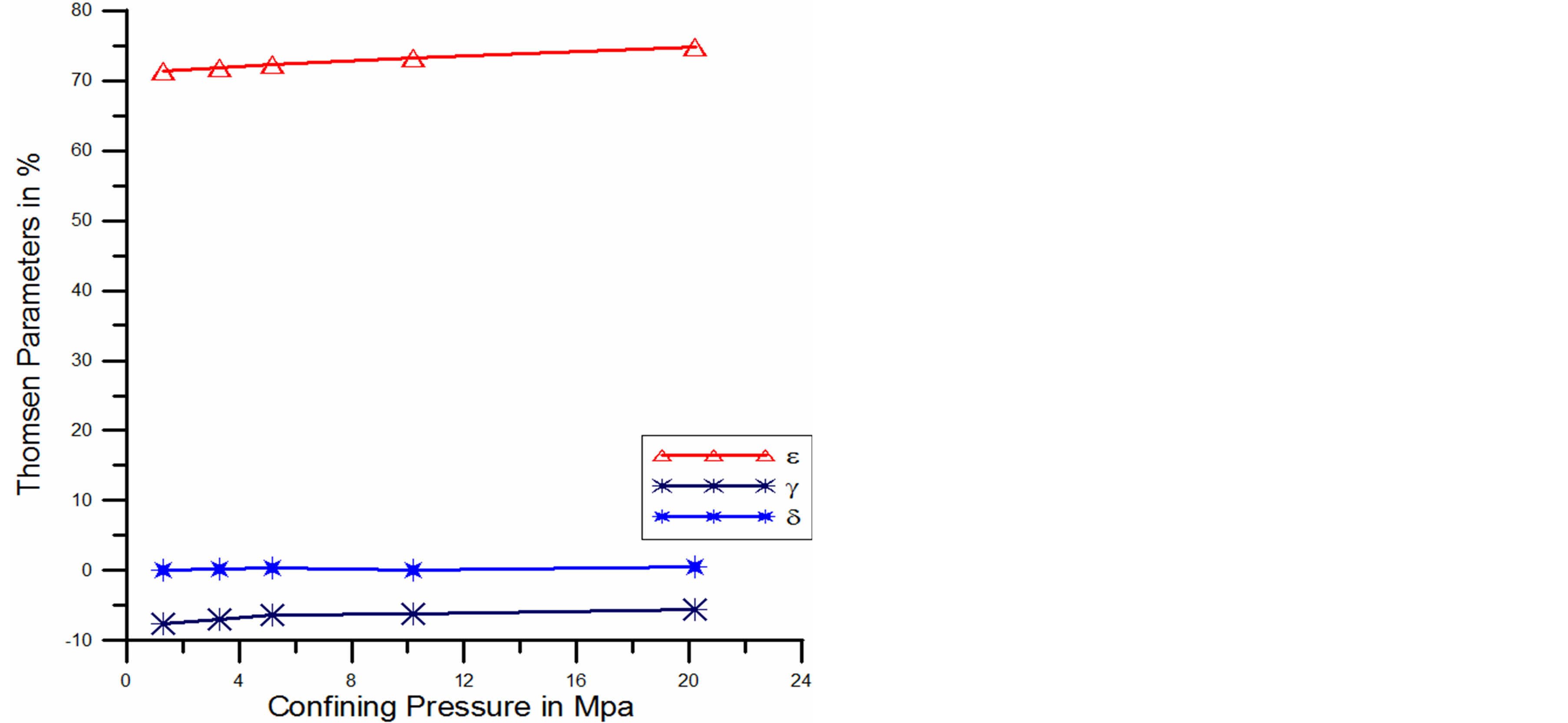
Figure 5. Comparison of Thomsen’s parameters as a function of confining pressure for sandyshale.

Figure 6. Comparison of Thomsen’s parameters as a function of confining pressure for saturated sandstone.
The analysis shows that the anisotropy parameters are increased as the confining pressures are increased for all the rock samples except saturated sandstone. Figure 6, shows that the anisotropy parameters are decreased when confining pressure are increase up to 15 Mpa, but again anisotropy parameters are increased with increasing confining pressure beyond 15 Mpa up to 40 Mpa for saturated sandstone.
3.1. Shale
Figure 7 shows that the Poisson’s ratio  and
and  varies as the confining pressure is raised. It has been observed that
  and
and  are slightly decreased as confining pressure is increased. The difference between
  and
and  remains approximately constant over the whole range of frequency, while
  remains approximately constant as the confining pressure is raised.
  is an indirect measure of the ratio of lateral to axial strain when the specimen is under uniaxial stress in the direction X. The high and almost constant value of
  indicated that the rock is very stiff and linearly elastic in the plane XY as consequence of the absence of voids and discontinuities in this plane.
 is an indirect measurement of the ratio of lateral strain to axial strain when the sample is subjected to uniaxial stress in the direction normal to the plane of isotropy Z
  is smaller than
  because the specimen is softer in the vertical direction than in the horizontal direction. The vertical direction is perpendicular to the foliation plane. Between the layers, there are discontinuities or void space filled with gas, liquid, or viscous organic material that increase the compliance of the rock in this direction. Thus the axial strain is larger than the lateral strain, resulting
 . Consequently, the axial strain rate is also less than the lateral strain rate, resulting in a decrease in
  as the pressure increased. The analysis of the sample shows that
  has similar behaviour to
 , however, the coefficients larger because the strain in the X direction is smaller than the strain in the Z direction, when the rock is compressed in the Z direction.
Figure 4 shows that the variation of velocity anisotropy as a function of confining pressure. Our analysis found that  remains approximately constant while confining pressure is increased, but
  and
and  are increased slightly as the pressure is increased.
3.2. Sandy Shale
Figure 5 shows that, the Vp anisotropy,  , is bigger that the Sh-anisotropy,
  within the confining pressure range. Oriented fractures affect the Vp-anisotropy more than the Vsh-anisotropy. When an Sh-wave propagates in the vertical and horizontal directions, the particle is polarized parallel to the plane of isotropy, and it always encounters more rigid material. However, when a P-wave propagates in the vertical and horizontal directions, the polarization of the particle and the direction of propagation are perpendicular and parallel to the plane of isotropy, respectively. The P-wave polarized in the vertical direction encounter softer material than the P-wave polarized in the horizontal direction. But our analysis shows that the Vp-anisotropy and Vsh-anisotropy are not approaching same value within our confining pressure range. That implies that the fracture of the specimen is not close within our pressure range. However, the anisotropic caused by preferred orientation of minerals, by fracture, and by layering are always due to the fact that the material is softer in the direction perpendicular to the direction of preferential orientation than in the direction
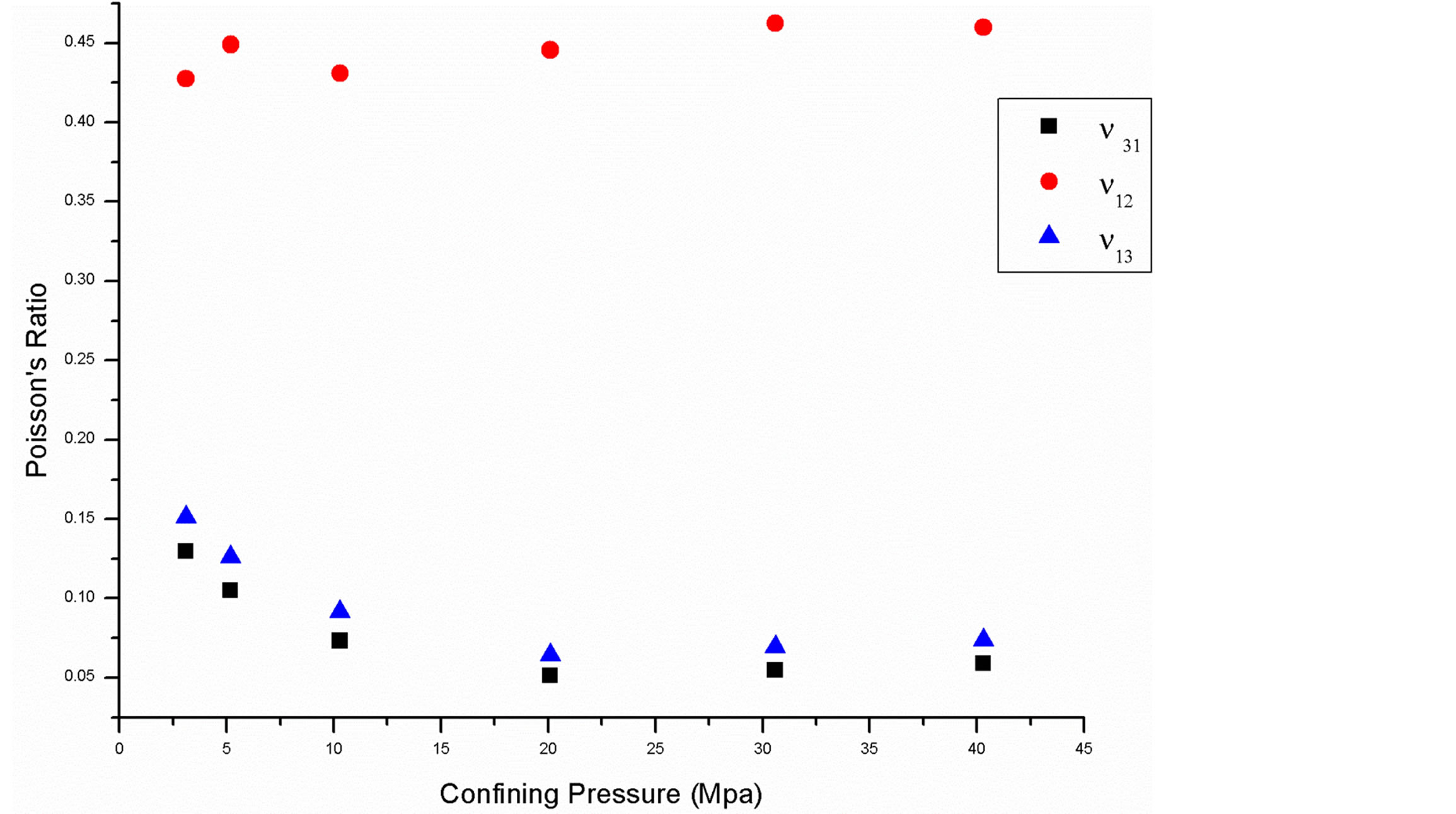
Figure 7. Relationship between Poisson’s ratio and confining pressure for shale.
parallel to it.
3.3. Dry and Saturated Sandstone
At low pressure, the Vp anisotropy , is higher than the Vsh anisotropy
 , and they trend to approach the same value at higher confining pressure. However,
  shows almost constant at all pressure. At higher pressure, the anisotropy is still controlled by the incomplete closures at the cracks.
After saturation Vp(0˚) and Vp(45˚) increase , while Vsv(0˚) decreases. Vp(0˚) and Vp(45˚) increase because the material is less compressible. A pore filled with fluid resists compression in a similar way when it is filled with solid material. The difference between Vp(0˚) for dry and for saturated sandstone decreases as the confining pressure is increased However, the difference between Vs(0˚) for dry and for saturated sandstones remain approximately constant The decrease in Vs(0˚) is caused by a significant increase in the bulk density, while C44 remains approximately constant (Figure 8). This explains why the difference between Vs(0˚) for dry and Vs(0˚) for saturated does not change as the confining pressure is increased. Vp(90˚) shows a significant increase after saturation. The significant increase is due to the polarization of the particle and the directions of propagation are perpendicular to the plane of isotropy, and fluid have a strong effect in this direction. The stiffness C33 shows a pronounced increase reaching the same value as C11. C44 remains approximately constant and C66 shows a slight decrease (Figure 8) after saturation.
After saturation, the P-wave anisotropy significantly decrease. However,  shows only a slight increase and remains increasing as the confining pressure is increased.
3.4. The Effect of Anisotropy on the Young’s Moduli and Poison’s Ratios
The strong effects of anisotropy parameters  and
and  on vertical and horizontal Young’s moduli and the Poisson’s ratios are shown in the Figures 9-16. The vertical Poisson’s ratio significantly decreases with
  for all four rock samples, while the horizontal Poisson’s ratio increases. On the other hand, both of the Young’s moduli increase with
  The anisotropy parameter
  has a completely different type of effect, the horizontal and vertical moduli show slightly constant at low
  but it increases as
  increased. The vertical and horizontal Poisson’s ratio show opposite effects with
 .
.
We showed that anisotropy has significant effect on the two key parameters; the Young’s modulus and the Poisson’s ratio. In fact there are two Young’s moduli and at least two Poisson’s ratios and they vary significantly with the magnitudes of the anisotropy parameters  and
and .
.
4. Conclusions
The study found that, the elastic anisotropy parameters are key factors which affect the estimation of hydrocarbon reservoir characterisation parameters. To estimate more accurate hydrocarbon reservoir characterisation parameters, we need vertical P-wave and S-wave velocities and three anisotropy parameters. With high quality and high resolution surface seismic data, we can reason-

Figure 8. Stiffness for dry and saturated sandstone specimens. The dashed curves show the stiffness in dry condition.

Figure 9. Relationship between vertical Young’s modulus and Epsilon .
.
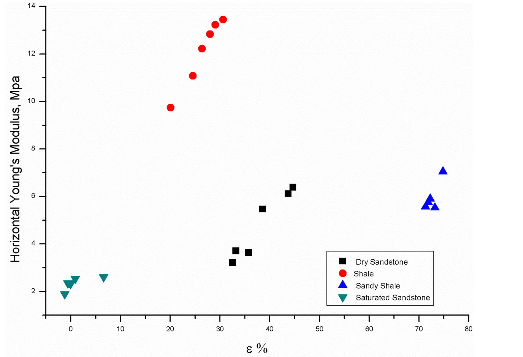
Figure 10. Relationship between horizontal Young’s modulus and Epsilo .
.
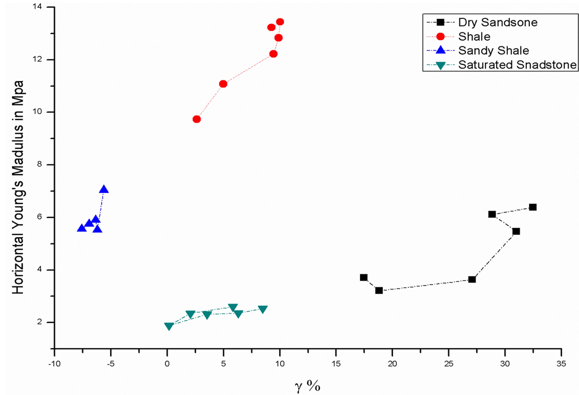
Figure 11. Relationship between horizontal Young’s modulus and Gamma 

Figure 12. Relationship between vertical Young’s modulus and Gamma .
.
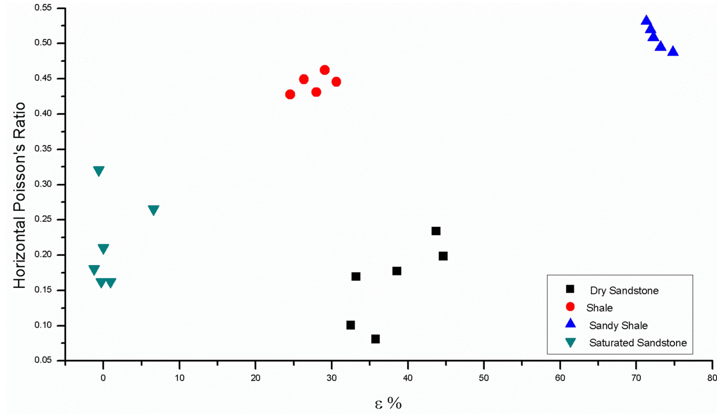
Figure 13. Relationship between horizontal Poisson’s ratio and Epsilon .
.
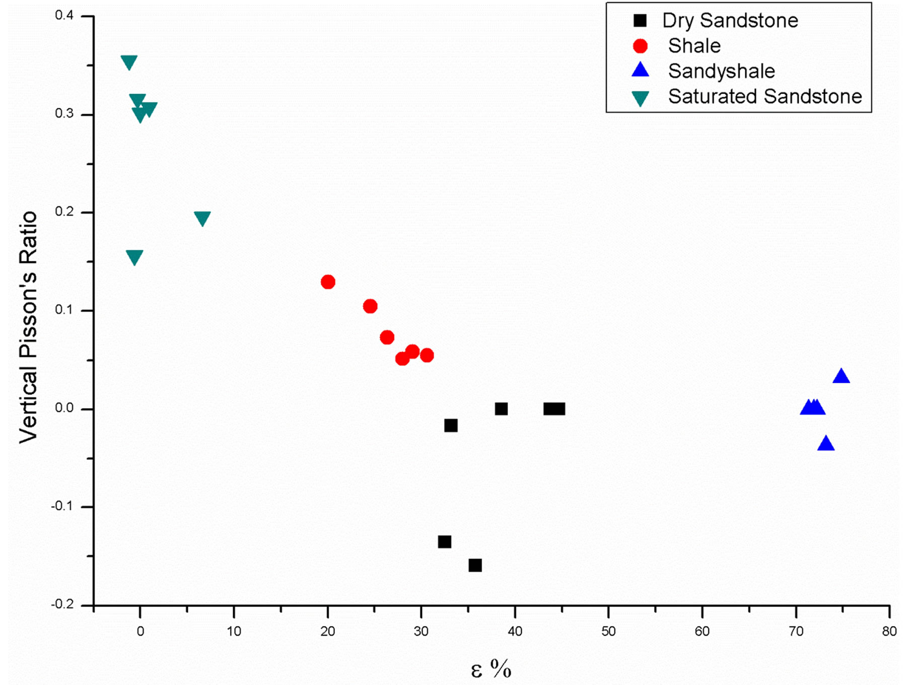
Figure 14. Relationship between vertical Poisson’s ratio and Epsilon .
.

Figure 15. Relationship between horizontal Poisson’s ratio and Gamma .
.
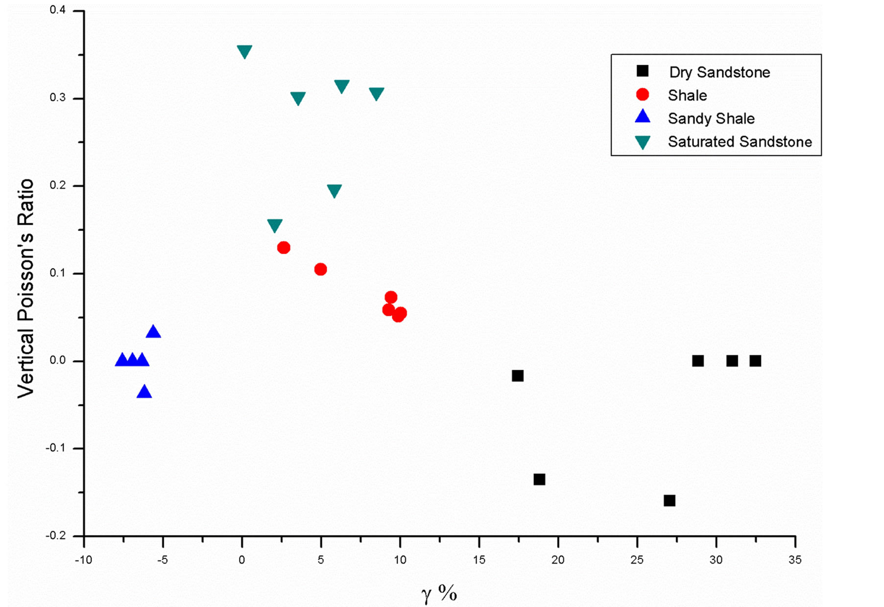
Figure 16. Relationship between vertical Poisson’s ratio and Gamma .
.
ably estimate  and
and , and for the remaining parameters, we must depend on the downhole data, wire line measurements including sonic scanner and borehole seismic such as walk away vertical seismic profiling. Our laboratory experiments on core samples will only be beneficial to obtain valid empirical relationships among some of the parameters to develop a starting model.
Thus through this study we proposed a prestack full waveform AVO inversion in a VTI medium constraining elastic parameters based on depth velocity analysis of P-wave surface seismic data and other information available.
This study also suggested that the Young’s moduli and Poisson’s ratios that the driller must have are the static moduli, not the dynamic moduli estimated through seismic experiment. The relationship established themselves in this study is laboratory based. The static moduli is larger than dynamic Young’s moduli by the factor 2 and it may vary basin to basin.
The initial model can be integrated by adding drilling and micro seismic monitoring, initial production, and estimated ultimate recovery data for updation.
Acknowledgements
We thank M/S Pandit Deendayal Petroleum University for supporting in preparation of manuscripts.
REFERENCES
[1] L. Thomsen, “Weak Elastic Anisotropy,” Geophysics, Vol. 51, No. 10, 1986, pp. 1954-1966. http://dx.doi.org/10.1190/1.1442051
[2] T. Alkhalifah and I. Tsvankin, “Velocity Analysis for Transversely Isotropic Media,” Geophysics, Vol. 60, No. 5, 1995, pp. 1550-1566. http://dx.doi.org/10.1190/1.1443888
[3] N. C. Banik, “Velocity Anisotropy of Shales and Depth Estimation in the North Sea Basin,” Geophysics, Vol. 49, No. 9, 1984, pp. 1411-1419. http://dx.doi.org/10.1190/1.1441770
[4] D. F. Winterstein, “Velocity Anisotropy Terminology for Geophysicists,” Geophysics, Vol. 55, No. 8, 1990, pp. 1070-1088. http://dx.doi.org/10.1190/1.1442919
[5] R. Brown and J. Korrigan, “On the Dependence of the Elastic Properties of a Porous Rock on the Compressibility of the Pore Fluid,” Geophysics, Vol. 40, No. 4, 1975, pp. 608-616. http://dx.doi.org/10.1190/1.1440551
[6] J. A. Hudson, “Overall Properties of a Cracked Solid,” Mathematical Proceedings of the Cambridge Philosophical Society, Vol. 88, No. 2, 1980, pp. 371-384. http://dx.doi.org/10.1017/S0305004100057674
[7] J. A. Hudson, “Wave Speeds and Attenuation of Elastic Waves in Material Containing Cracks,” Geophysical Journal International, Vol. 64, No. 1, 1981, pp. 133-150. http://dx.doi.org/10.1111/j.1365-246X.1981.tb02662.x
[8] J. A. Hudson, “Overall Elastic Properties of Isotropic Materials with Arbitrary Distribution of Circular Cracks,” Geophysical Journal International, Vol. 102, No. 2, 1990, pp. 465-469. http://dx.doi.org/10.1111/j.1365-246X.1990.tb04478.x
[9] J. A. Hudson, “Crack Distribution Which Accounts for a Given Seismic Anisotropy,” Geophysical Journal International, Vol. 104, No. 3, 1991, pp. 517-521. http://dx.doi.org/10.1111/j.1365-246X.1991.tb05698.x
[10] J. A. Hudson, E. Liu and Crampin, “The Mechanical Properties of Materials Which Interjected Cracks and Pores,” Geophysical Journal International, Vol. 124, No. 1, 1996, pp. 105-112. http://dx.doi.org/10.1111/j.1365-246X.1996.tb06355.x
[11] T. Mukerji and G. Mavo, “Pore Fluid Effects on Seismic Velocity in Anisotropic Rocks,” Geophysics, Vol. 59, No. 2, 1994, pp. 233-244. http://dx.doi.org/10.1190/1.1443585
[12] L. Thomsen, “Elastic Anisotropy Due to Aligned Cracks in Porous Rock,” Geophysical Prospecting, Vol. 43, No. 6, 1995, pp. 805-829. http://dx.doi.org/10.1111/j.1365-2478.1995.tb00282.x
[13] T. D. Jones, “Wave Propagation in Porous Rock and Models for Crustal Structures,” Ph.D. Thesis, Standford University, 1983.
[14] N. M. Lucet and P. A. Tarif, “Shear—Wave Birefringence and Ultrasonic Shear Wave Attenuation Measurements,” SEG Annual Meeting, Anaheim, 30 October-3 November 1988, pp. 922-924.
[15] M. Zamora and J. P. Porier, “Experimental Study of Acoustic Anisotropy and Birefringence in Dry and Saturated Fontainebleau Sandstone,” Geophysics, Vol. 55, No. 11, 1990, p. 1455. http://dx.doi.org/10.1190/1.1442793
[16] B. E. Hornby, “Experimental Laboratory Determination of the Dynamic Elastic Properties of Wet, Drained Shales,” Journal of Geophysical Research: Solid Earth, Vol. 103, No. B12, 1998, pp. 29945-29964.
[17] Z. Wang, “Seismic Anisotropy in Sedimentary Rocks,” Part 1: A Single-Plug Laboratory Method,” Geophysics, Vol. 67, No. 5, 2002, pp. 1415-1422. http://dx.doi.org/10.1190/1.1512787
[18] K. Bjørlykke, “Clay Mineral Diagenesis in Sedimentary Basins—A Key to the Prediction of Rock Properties. Examples from the North Sea Basin,” Clay Minerals, Vol. 33, 1998, pp. 15-34.
[19] M. S. Sam and A. Andrea, “The Effect of Clay Distribution on the Elastic Properties of Sandstones,” Geophysical Prospecting, Vol. 49, No. 1, 2001, pp. 128-150. http://dx.doi.org/10.1046/j.1365-2478.2001.00230.x
[20] Z. Wang, “Seismic Anisotropy in Sedimentary Rocks, Part 2: Laboratory Data,” Geophysics, Vol. 67, No. 5, 2002, pp. 1423-1440. http://dx.doi.org/10.1190/1.1512743
[21] J. M. Leslie and D. C. Lawton, “A Refraction Seismic Field Study to Determine the Anisotropic Parameters of Shales,” The Leading Edge, Vol. 17, No. 8, 1998, pp. 1127-1129. http://dx.doi.org/10.1190/1.1438105
[22] G. Mavko, T. Mukerji and J. Dvorkin, “Rock Physics Handbook: Tools for Seismic Analysis in Porous Media,” Cambridge University Press, 1998.
[23] F. R. Pena, “Elastic Properties of Sedimentary Anisotropic Rocks,” Dissertation, Massachusetts Institute of Technology, 1998, pp. 19-26.