International Journal of Geosciences
Vol.4 No.9(2013), Article ID:40224,7 pages DOI:10.4236/ijg.2013.49123
A New Approach for Smoothing Soil Grain Size Curve Determined by Hydrometer
Geology Department College of Science, University of Mosul, Mosul, Iraq
Email: *thanoon53@yahoo.com
Copyright © 2013 Mohammed Q. H. AL-Jumaily, Thanoon H. AL-Dabbagh. This is an open access article distributed under the Creative Commons Attribution License, which permits unrestricted use, distribution, and reproduction in any medium, provided the original work is properly cited.
Received July 19, 2013; revised August 22, 2013; accepted September 23, 2013
Keywords: Hydrometer; Soil Mechanics; Grain Size
ABSTRACT
In hydrometer analysis for soil grain size distribution, usually, the grains passing sieve No. 200 (<0.074 mm) are used. However, the hydrometer results occasionally give diameters greater than 0.074 mm. This event causes a mismatch in the curve of grain size distribution obtained from sieving and hydrometer methods. Hence, a new approach is proposed for smoothing soil grain size curve determined by hydrometer using Excel-2007 with simple statistical methods. The treatments show that in case of large sizes, there are big differences between the values of soil grain diameters smoothed by Excel-2007 in comparison and the values measured by references. These differences generally decrease with decreasing soil grain size diameters. The statistical treatments also divulge whether the hydrometer results are accurate or not. Furthermore, a general equation has been derived to estimate values of K factor, which is used for calculating the grain diameters in hydrometer analysis. The equation can be applied for any specific gravity of soils and for wide range temperatures.
1. Introduction
Most soil mechanics laboratories run soil grain size analysis as a routine test. The distribution of particle sizes, which is larger than 0.074 mm (retained on sieve No. 200), is determined by sieving method, while the distribution of particle sizes smaller than 0.074 mm is determined by a sedimentation process using hydrometer method.
Lambe [1] stated that the hydrometer method is based on Stokes’ Equation for the velocity of a freely failing sphere; the definition of particle diameter of a sphere of the same density falls at the same velocity as the particle in equation. The first of the above assumptions can be practically satisfied by limiting the maximum concentration of soil in the suspension. No more than 50 gm of dry soil are used in 1000 cc of suspension; the effects of interference are negligible. It is known that the most soil particles comprise of flaky shapes, principally in case of fine soils. Also, the soil particles are not exactly equal in density. Moreover, there are many other factors affecting the accuracy of the hydrometer results discussed in details by [1].
Fredlund et al. [2] present two mathematical forms to represent grain size distribution curves for well-graded soils and gap-graded soil. Lu et al. [3] provides a rigorous analysis on the accuracy of Stokes’ Equation for calculating particle-size distributions of non-spherical finegrained clay particles.
Keller and Gee [4] compare the hydrometer method (D422) for PSA (particle-size analysis) of the American Society of Testing Materials (ASTM) with the hydrometer method published by the Soil Science Society of America (SSSA).
Stefano et al. [5] compare laser diffraction method (LDM) with the sieve-hydrometer method (SHM). A simplified approach is presented and evaluated by Bedaiwy [6]. The approach simply bases on the determination of he directly on the geometric center (g.c.) of the hydrometer bulb rather than the center of buoyancy, and he is measured as the distance from the reading mark on the hydrometer stem to that geometric center.
The difficulty experienced by all soil mechanics laboratories is the large sizes of soil grains (greater than 0.074 mm) obtained from the hydrometer method, even though the soil grains pass sieve No. 200 (<0.074 mm). This problem causes a mismatch in the curve obtained from sieving analysis and that obtained from hydrometer analysis results. Moreover, the problem causes a lack of accuracy in the hydrometer results. For all these reasons, the study attempts to solve this problem by smoothing soil grain size curves determined by hydrometer using Excel-2007 with simple statistical methods.
2. Treatments by Excel-2007
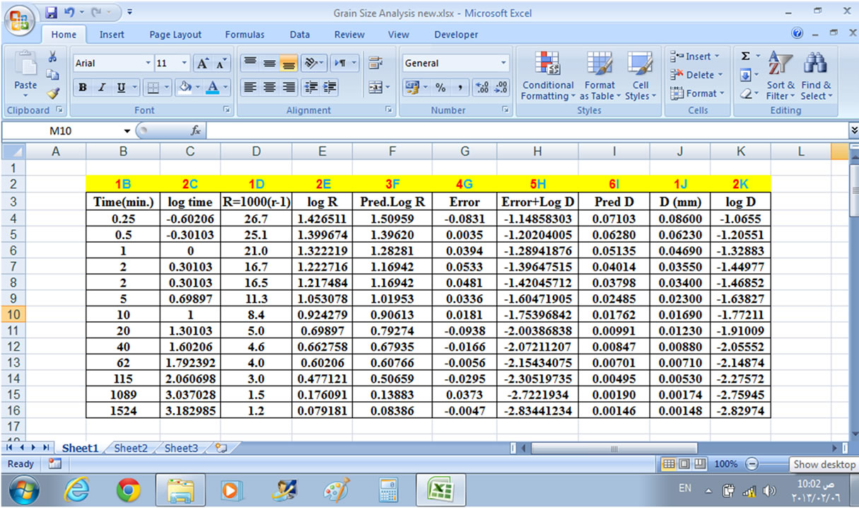
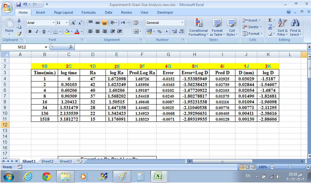
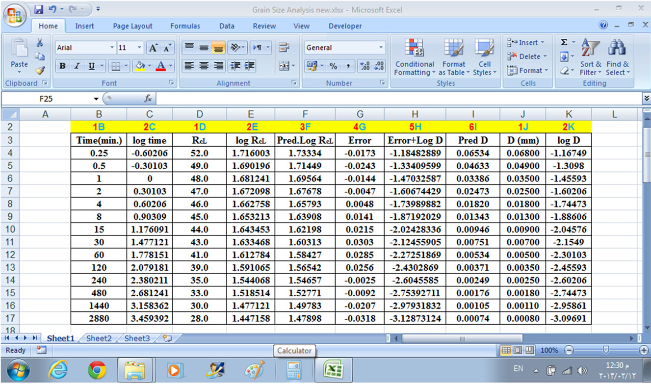
To clarify these treatments, the hydrometer data for Lambe [1], with hydrometer specific gravity range (0.995 - 1.05), have been used (Figure 1). Note that in Figure 1(a): the yellow row (i.e. row number two) shows red colored numbers referring to step-number and the blue colored letters referring to column-number.
The treatment process steps are as follows:
Step 1: Enter the time in minutes (1B), hydrometer readings (1D), and diameters in mm (1J) (Figure 1(a)).
Step 2: Around the values of time, hydrometer reading, and diameter to logarithmic (Log10) values (2C), (2E), and (2K) respectively (Figure 1(a)). Draw scatter plots between log hydrometer reading and log diameter on the (Y-axis) with log time on the (X-axis) as shown in Figure 1(b). This figure shows that the fluctuation in log hydrometer reading curve is different from the log diameter curve. This means that the log diameter curve is not affected by the same influences that affect the log hydrometer reading curve.
Step 3: Draw a straight line curve between log hydrometer reading on the (Y-axis) and log time on the (X-axis) (Figure 1(c)). To determine the slope and intercept for this straight line use the equation shown in Figure 1(c) to predict the calculated values for the log hydrometer reading (3F) (Figure 1(a)).
Step 4: Calculate the difference (Error) between log hydrometer reading, and predicted log hydrometer reading by subtracting the second values from the first (4G) (Figure 1(a)).
Step 5: Add the error values to log diameter values (5H) (Figure 1(a)).
Step 6: Change the values that have been obtained in Step 5 from logarithmic numbers to ordinary numbers as predicted diameter values (6I) (Figure 1(a)). Next draw scatter plots between log hydrometer reading and log predicted diameter on the (Y-axis) with log time on the (X-axis), as shown in Figure 1(d). This figure shows the same fluctuation in both log hydrometer reading and log predicted diameter. This indicates that log predicted diameter curve are affected by the same influences which affects the log hydrometer reading curve. To demonstrate the importance of these processes on the Lamb 1951 results, the predicted results one compared with the Lamb results, as shown in Table 1 and Figures 1(e) and (f). These two figures show that the hydrometer curve in Figure 1(e) does not run smoothly and continuously with the sieve curve in comparison with the predicted result curve of Figure 1(f).
To clarify these treatments, other data were used for hydrometer ASTM 152-H, shown in Figure 2(a) of Krishna [7]. The results are represented in Figures 2(b), (c), and (d). The predicted Krishna [7] results are shown in Table 2 and Figures 2(e) and (f). These two figures show that in case of the smallest sizes the differences between the two curves are less than the differences in Figures 1(e) and (f). However, Figure 2(f) shows that the smooth curved is relatively better than the curve in Figure 2(e).
Other hydrometer results, ASTM 152-H, for Das [8] are treated here. The results are shown in Figures 3(a) to (f). It is clear from Figure 3(e) that there is a good matching between the results before and after treatments.
The hydrometer data, 151H, for CEEN 162 [9] are shown in Figure 4. It appears that there is an excellent matching between the CEEN 162 results before and after treatments due to the high accuracy results. Therefore there is no need to draw the related figures for this almost perfect data.
Finally, the hydrometer results data, ASTM 152-H, for David [10] are represented in Figure 5. The figure shows that there is a bad correlation between log hydrometer reading and log time due to errors in hydrometer readings as shown clearly in column (1D).
The above treatment results clearly show whether the hydrometer readings are accurate or not.
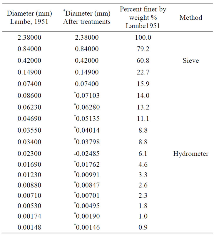
Table 1. Lambe, 1953, results before and after treatments [1].
 (a)
(a)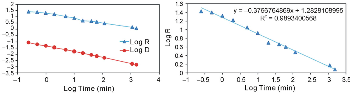 (b)
(b)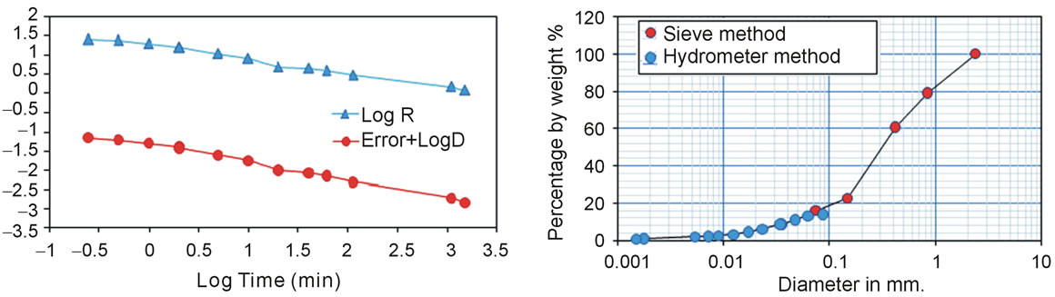 (c)
(c)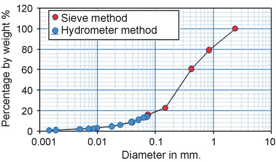 (d)
(d)
Figure 1. hydrometer results data for Lambe [1]. (a): The smoothing treatments processes by Excel-2007. (b): Scatter plots between log hydrometer reading and log diameter with log time before treatments. (c): Straight line equation between log hydrometer reading and log time. (d): Scatter plots between log hydrometer reading and log predicted diameter with log time after treatments. (e): Grain size distribution curve before treatments. (f): Grain size distribution curve after treatments.
 (a)
(a)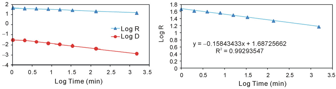 (b)
(b)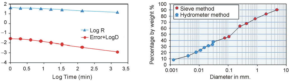 (c)
(c)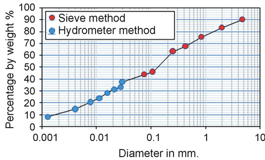 (d)
(d)
Figure 2. Hydrometer results data for Krishna [7]. (a): The smoothing treatments processes by Excel-2007. (b): Scatter plots between log Hydrometer reading and log diameter with log time before treatments. (c): Straight line equation between log hydrometer reading and log time. (d): Scatter plots between log Hydrometer reading and log predicted diameter with log time after treatments. (e): Grain size distribution curve before treatments. (f): Grain size distribution curve after treatments.
 (a)
(a)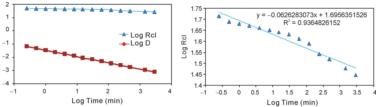 (b)
(b)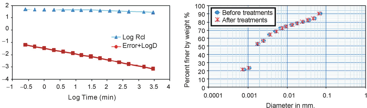 (c)
(c)
Figure 3. Hydrometer results data for Das [8]. (a): The smoothing treatments processes by Exce-2007. (b): Scatter plots between log Hydrometer reading and log diameter with log time before treatments. (c): Straight line equation between log hydrometer reading and log time. (d): Scatter plots between log Hydrometer reading and log predicted diameter with log time after treatments. (e): hydrometer grain size distribution curve before and after treatments.
3. K Factor
The value of K is a very important factor in hydrometer analyzing method to calculate soil grain diameters. The old conventional method uses confidential tables to find K factor by means of temperature and specific gravity of soil. In this study, the following general equation has been derived numerically upon K tables to determine the values of K as:
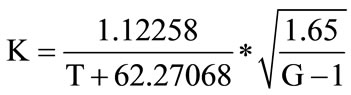
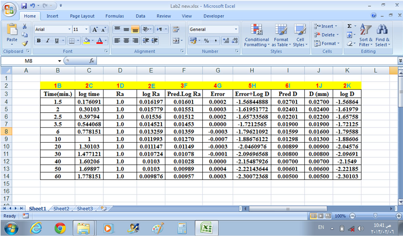
Figure 4. Shows the smoothing treatments for CEEN 162 [9] hydrometer analysis data by Excel-2007.

Figure 5. Shows the hydrometer results data for David [10] by Excel-2007 with a bad correlation.
whereT = Temperature in Celsius and G = Specific gravity of soil solids.
The equation can be applied for any specific gravity of soil within known ranges and for a temperature range from 10 to 40 Celsius.
4. Results and Conclusions
The statistical treatment results using Excel-2007 show that there are big differences between the values of soil grain diameters determined by this method and those measured by references. These differences may be due to the lack of the time accuracy, especially at the beginning of the test. In addition, the three assumptions for Stokes’ equation do not match exactly with soil properties. The Excel-2007 results give a smoother and more matching grain size distribution curve.
In case of decreasing soil grain size particles, these
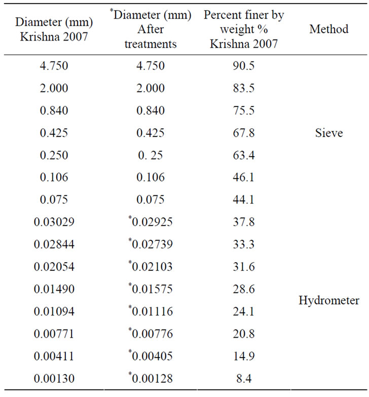
Table 2. Krishna, 2007, results before and after treatments [7].
differences decreases strongly because of the high correlation between log time and log hydrometer reading.
The treatments will reveal whether the hydrometer results are accurate or not.
A general equation has been derived to obtain values of K, which is a very important factor for determining soil grain diameters in hydrometer analysis. This equation may be applied for any specific gravity of soil and for a wide temperature range.
REFERENCES
- L. T. William, “Soil Testing for Engineers,” Chapter IV, John Wiley & Sons, Inc., New York, London, Sydney, 1951, pp. 29-42.
- M. D. Fredlund, D. G. Fredlund and G. W. Wilson, “An Equation to Reptesent Grain-Size Distribution,” Canadian Geotechnical Journal, Vol. 37, No. 4, 2000, pp. 817- 827. http://dx.doi.org/10.1139/t00-015
- N. Lu, G. H. Ristow and W. J. Likos, “The Accuracy of Hydrometer Analysis for Fine-Grained Clay Particles,” ASTM Geotechnical Journal, Vol. 23, No. 4, 2000, pp. 487-495.
- J. M. Keller and G. W. Gee, “Comparison of American Society of Testing Materials and Soil Science Society of America Hydrometer Methods for Particle-Size Analysis,” Soil Science Society of America Journal, Vol. 70, No. 4, 2006, pp. 1094-1100. http://dx.doi.org/10.2136/sssaj2005.0303N
- C. Di Stefano, V. Ferro and S. Mirabile, “Comparison between Grain-Size Analyses Using Laser Diffraction and Sedimentation Methods,” Biosystems Engineering, Vol. 106, No. 2, 2010, pp. 205-215. http://dx.doi.org/10.1016/j.biosystemseng.2010.03.013
- M. N. A. Bedaiwy, “A Simplified Approach for Determining the Hydrometer’s Dynamic Settling Depth in Particle-Size Analysis,” Catena, Vol. 97, 2012, pp. 95-103. http://dx.doi.org/10.1016/j.catena.2012.05.010
- R. Krishna, “Engineering Properties of Soils Based on Laboratory Testing,” UIC 44 Experiment 6 Grain Size Analysis (Sieve and Hydrometer), University of Nebraska, Lincoln, 2007, pp. 44-59.
- B. M. Das, “Soil Mechanics Laboratory Manual,” 6th Edition, Oxford, New York, 2002, p. 277.
- CEEN 162, “Geotechnical Engineering—Laboratory Session No. 2. Grain Size Determination (Hydrometer Method),” Atterberg Limits, Sand Equivalent Test, p. 24.
- B. David, 2003. “Physical and Plasticity Characteristics Experiments #1-5,” CE 3143, pp. 13-17.
NOTES
*Corresponding author.