International Journal of Geosciences
Vol.4 No.4(2013), Article ID:33370,22 pages DOI:10.4236/ijg.2013.44067
Hyperbolic Velocity Model
Paradigm Geophysical, Herzliya, Israel
Email: igor.ravve@pdgm.com, zvi.koren@pgdm.com
Copyright © 2013 Igor Ravve, Zvi Koren. This is an open access article distributed under the Creative Commons Attribution License, which permits unrestricted use, distribution, and reproduction in any medium, provided the original work is properly cited.
Received March 27, 2013; revised April 29, 2013; accepted May 26, 2013
Keywords: Velocity Models; Velocity Transforms; Sediments
ABSTRACT
Asymptotically bounded velocity profiles describe the vertical velocity variations in compacted sediments in a more realistic way than unbounded velocity models, and allow presenting the subsurface by a smaller number of thicker layers. The first and the simplest asymptotically bounded model is the Hyperbolic velocity profile proposed by Muscat in 1937, and our paper is an extension of this early study. The Hyperbolic model has an advantage over other bounded models: The velocity increases with depth and approaches the limiting value with a more smooth and gradual rate. We derive the time-depth relationships, forward and backward transforms between the instantaneous velocity profile and the effective models (average, RMS and fourth order average velocities), study the trajectories for pre-critical and post-critical curved rays and derive the equations for traveltime, lateral propagation and arc length. We compare the ray paths obtained with the Hyperbolic model and with the other bounded velocity profiles.
1. Introduction
The Hyperbolic velocity model was first proposed by Muscat [1] and published in 1937. However, since then the model was not extensively studied and is unjustifiably ignored in the literature. The objective of this research is to extend the original study and to correct the inaccuracies. We show the place of the Hyperbolic model among the other asymptotically bounded models, analyze its basic relationships and attempt to develop a complete theory.
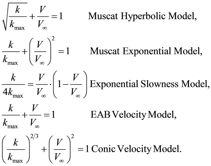
Asymptotically bounded velocity models describe the velocity profile in compacted sediments, where the velocity gradually increases with depth and eventually approaches a limiting value. These models make it possible to describe a vertical velocity profile with a smaller number of intervals as compared to the classical unbounded models, such as linear velocity vs. depth [2,3], unbounded exponent [4], linear slowness [5], “sloth” (linear variation of slowness squared), e.g., [6], parabolic model [7,8], Faust velocity model [9,10] with a reference depth and different root indices. The unbounded models are described by two parameters: the instantaneous velocity at the top interface  and the vertical velocity gradient
  at the same level. The Faust model includes also the root index n, normally
 . Asymptotically bounded models require an additional parameter: the limiting value of velocity
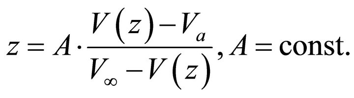
  at infinite depth. Two models of this family were studied by Ravve and Koren: the Exponential asymptotically bounded model [11,12] and the Conic model [13]. The asymptotically bounded profiles can be used, in particular, as velocity trend functions for the constrained velocity inversion with the best (e.g., least-squares) fit of the input data [14]. Examples of asymptotically bounded models are presented below. For each model, we first give the original formulation of the velocity profile as it appears in the original works by the authors, and then we convert it to a canonical form in terms of the “standard” parameters
  and
and . Parameter
  means the instantaneous velocity range,
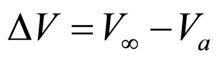 .
.
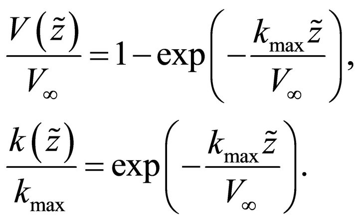
• The Hyperbolic velocity model by Muscat [1],
 (1)
(1)
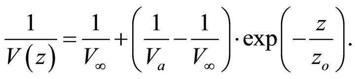
In our notation, the Hyperbolic profile reads
 (2)
(2)
• The Exponential velocity model by Muscat [1],
 (3)
(3)
We convert it to our notation,
 (4)
(4)
where the parameters are
 (5)
(5)
• The Exponential slowness model [5,15],
 (6)
(6)
It can be converted to canonic form,
 (7)
(7)
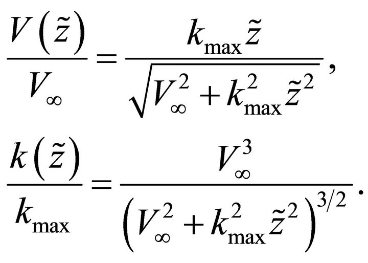
• The Exponential asymptotically bounded (EAB) velocity model [11,12],
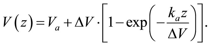 (8)
(8)
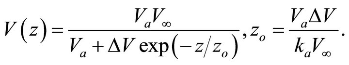
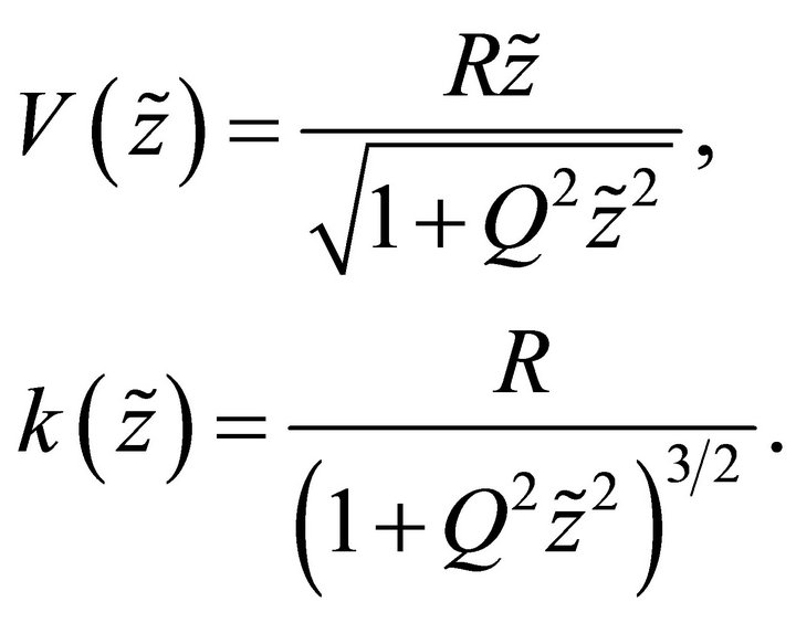
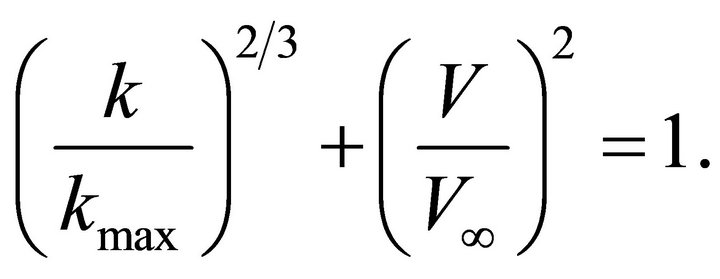
• The Conic velocity model [13],
 (9)
(9)
where
 (10)
(10)
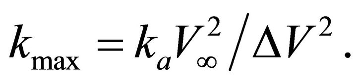
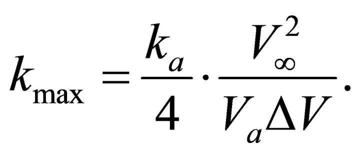
A detailed review on unbounded and bounded velocity models is given by Kaufman [16]. Figure 1 shows graphs of the instantaneous velocity vs. depth for the five asymptotically bounded velocity models mentioned above.
For all models, we assume the same velocity profile parameters: . The vertical gradients of the velocity vs. depth are plotted in Figure 2. It is interesting to note that among the five models presented, the Muscat Hyperbolic model (Equation (1) and grey line on the plot) approaches the limiting value
  in the slowest and the most gradual manner. The “second slow” is the Conic velocity model (red line), and the “third slow” is the EAB model (blue line). An asymptotically bounded model can be characterized by its gradient-velocity relationship, which is actually the governing differential equation of the velocity model.
This paper is structured as follows. We define the Hyperbolic model using 1) the original Muscat [1] formulation—depth vs. velocity, 2) the physical parameters: maximum gradient R, length scale  and vertical shift h, and 3) the “technical” or geophysical parameters: top interface velocity
 , top gradient
  and asymptotic velocity
 . We introduce the dimensionless asymptotic factor
  that simplifies the transform equations. First
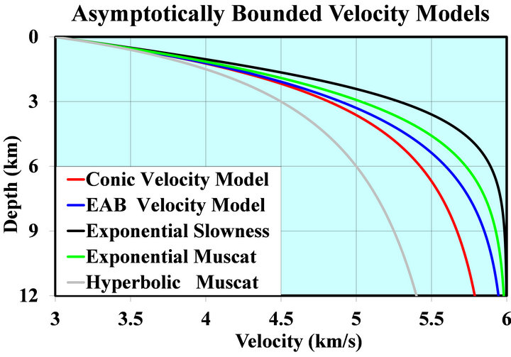
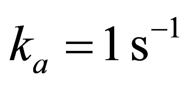
Figure 1. Asymptotically bounded velocity models: Muscat hyperbolic model, Muscat exponential model, the Exponential slowness model, the Exponential asymptotically bounded model and the Conic model: Velocity vs depth. For all models, the profile parameters are: the top interface velocity Va = 3 km/s, the top gradient ka = 1 s−1 and the asymptotic velocity V∞ = 6 km/s.
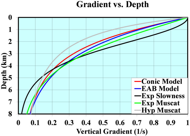
Figure 2. Vertical gradients vs. depth for asymptotically bounded velocity models.
we derive the time-depth and the depth-time relationships. Next we proceed to forward transforms from the instantaneous velocities to the effective models, such as the average, the RMS and the fourth order average velocity. Then we study the inversion problems, considering the inversion with the instantaneous velocities and gradients, and the inversion with the effective models, i.e., the average or the RMS velocities given vs. time or depth. Next we comment on the two types of curved rays existing in all asymptotically bounded models, depending on the initial take-off angle, and derive the trajectories of the ray paths for the Muscat velocity profile. For both types of the curved rays we derive the lateral propagation, the traveltime and the arc length.
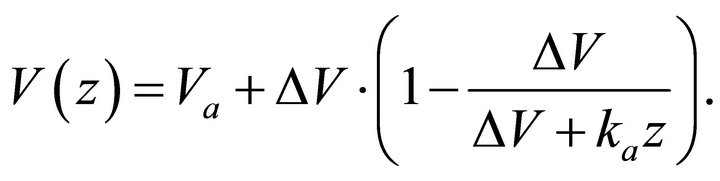
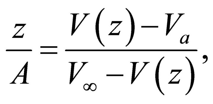
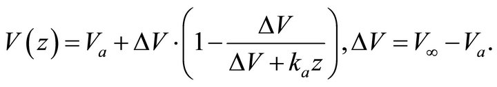
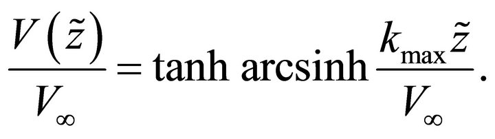
2. The Hyperbolic Velocity Profile
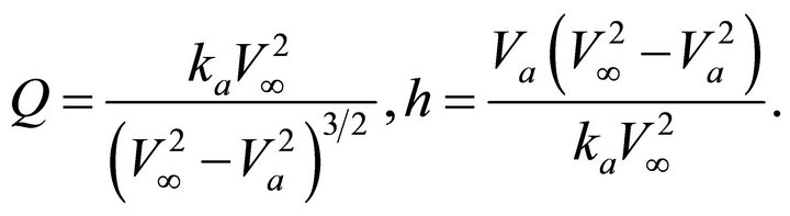
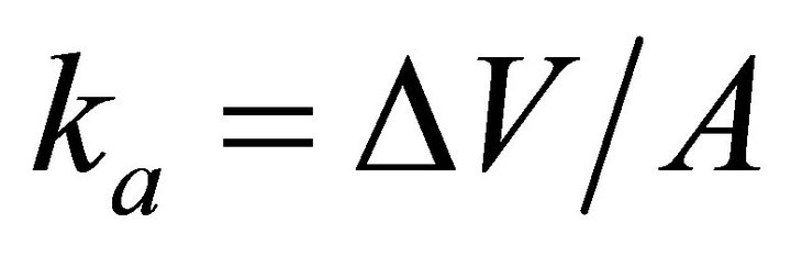
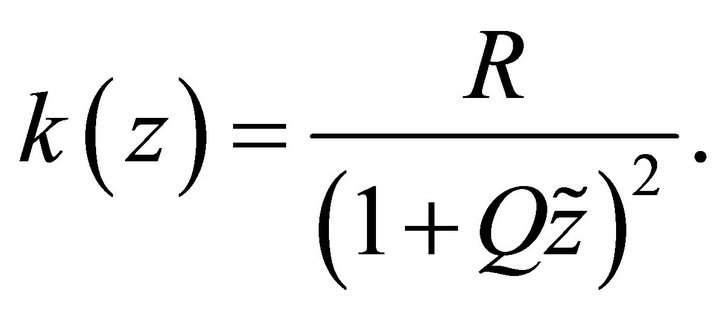
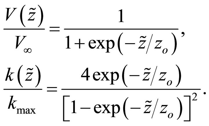
Muscat [1] defined the Hyperbolic model by
 (11)
(11)
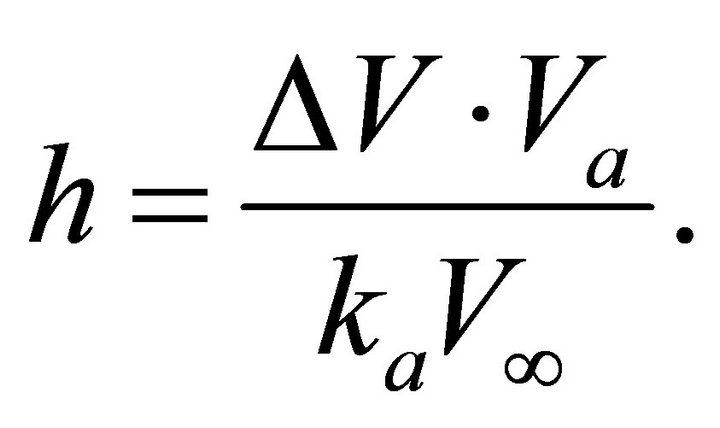
where V is the instantaneous velocity, z is depth measured from the top interface,  is the top interface velocity, A is the characteristic distance (scale) that affects the top gradient
 , and
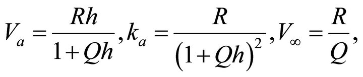
, and  is the asymptotic velocity. Inverting Equation (1), we obtain
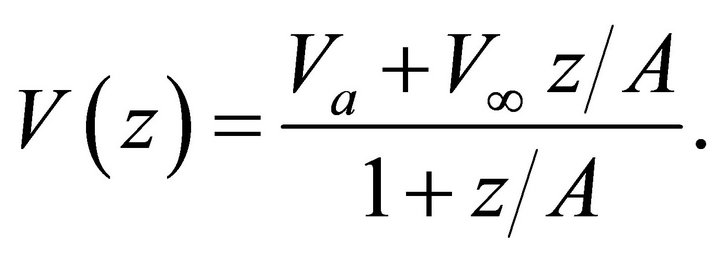 (12)
(12)
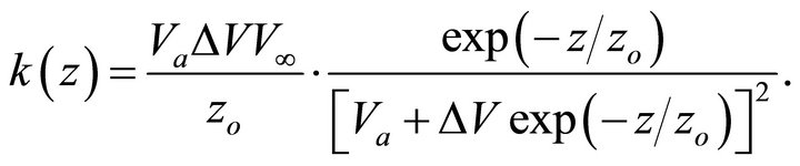
The velocity gradient becomes
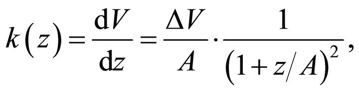 (13)
(13)
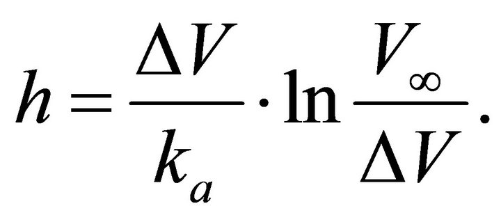
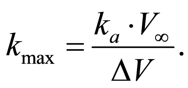
where  At
At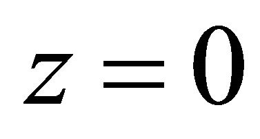 , the top gradient is
 . Therefore,
 and
and 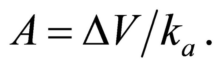 (14)
(14)
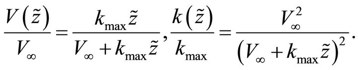
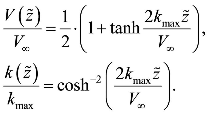
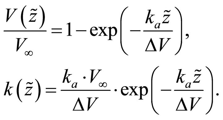
Introduce Equation (14) into Equation (13). In our notation, the Hyperbolic profile reads
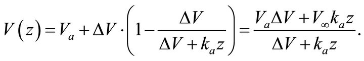 (15)
(15)
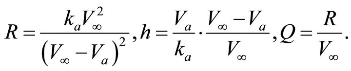
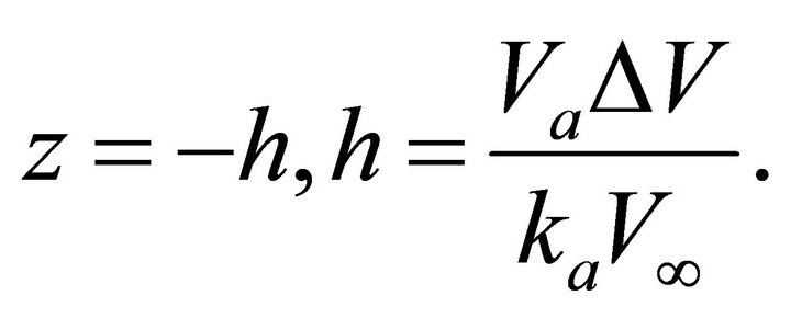
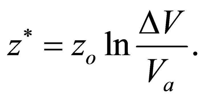
We call values  and
and  the technical parameters of the profile. At a definite height above the earth surface (above the upper interface), where
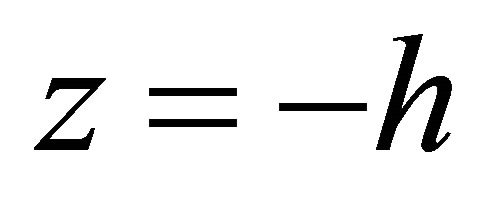 , the instantaneous velocity vanishes. According to Equation (15),
 (16)
(16)
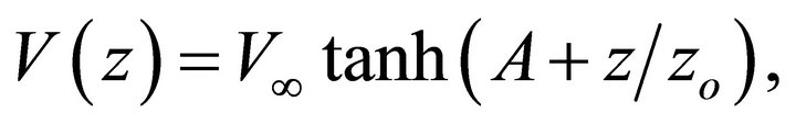
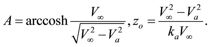
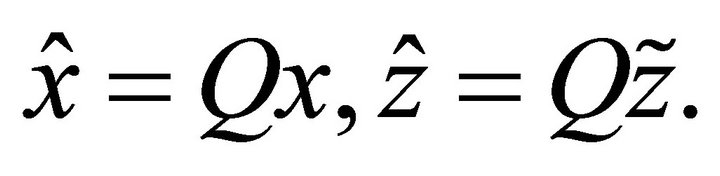
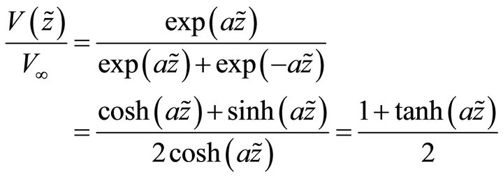
Introduce the absolute frame , where the instantaneous velocity vanishes at the origin
 . Parameter
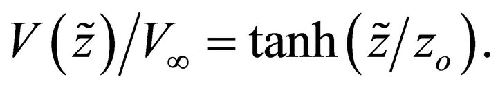
  is the shift between the two frames of reference. In the absolute frame, the velocity profile simplifies to
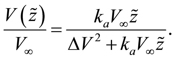
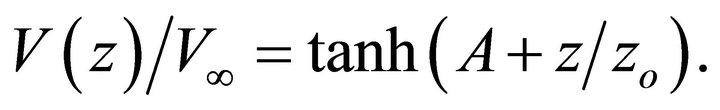
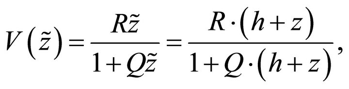 (17)
(17)
where
 (18)
(18)
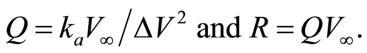
We call values  and
and  the physical parameters of the profile. Note that the linear velocity profile, where the ray trajectories are circular arcs, is a particular case of the Hyperbolic model with
  and
and , in such way that their product
  remains a finite value, and parameter
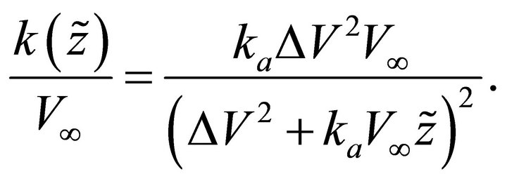
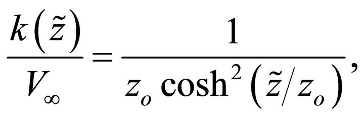
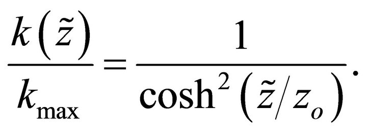
  becomes the constant velocity gradient of the linear model. The velocity gradient of the Hyperbolic model reads
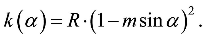
 (19)
(19)
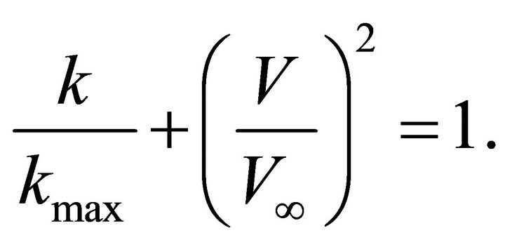
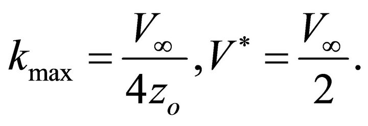
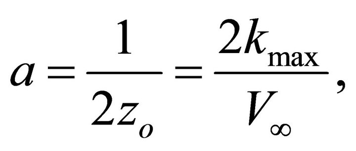
At the absolute origin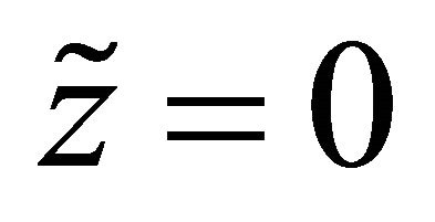 , the velocity gradient reaches its maximum value
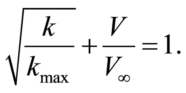
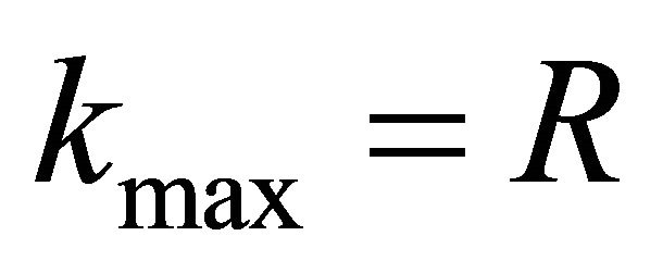 . Comparing Equations (17) and (19), we conclude that
 (20)
(20)
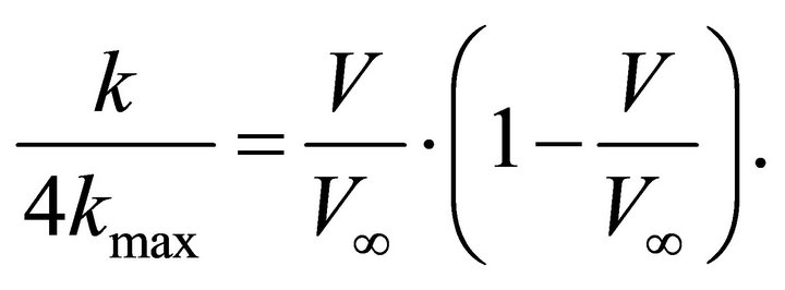
Equation (20) is the governing differential equation of the Hyperbolic velocity profile. It can be used to plot the gradient-velocity diagram. Such diagrams for several asymptotically bounded velocity models are studied in Appendix A.
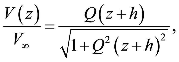
Introduce the normalized (dimensionless) velocity![]() , the normalized gradient
, the normalized gradient  and the normalized absolute depth
 ,
,
 (21)
(21)
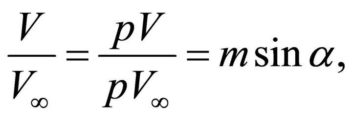
Note that parameter Q is the reciprocal characteristic length. With these notations, the Hyperbolic velocity profile simplifies to
 (22)
(22)
The technical parameters of the velocity profile are related to the physical parameters,
 (23)
(23)
The inverse relationship is
 (24)
(24)
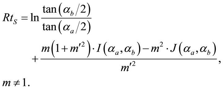
3. Asymptotic Factor
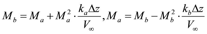
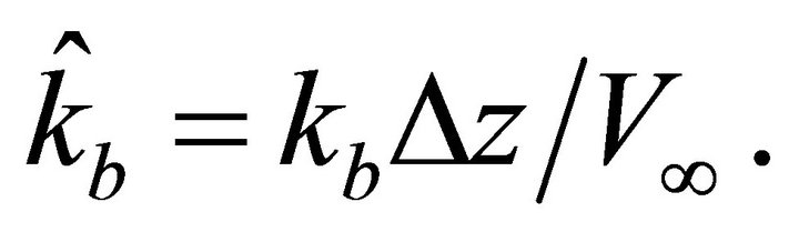
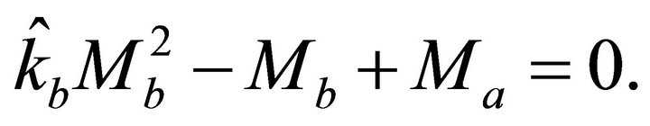
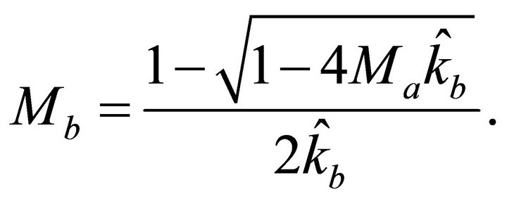
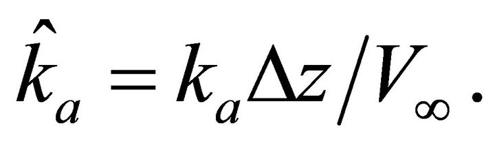
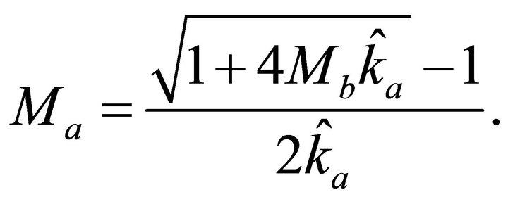
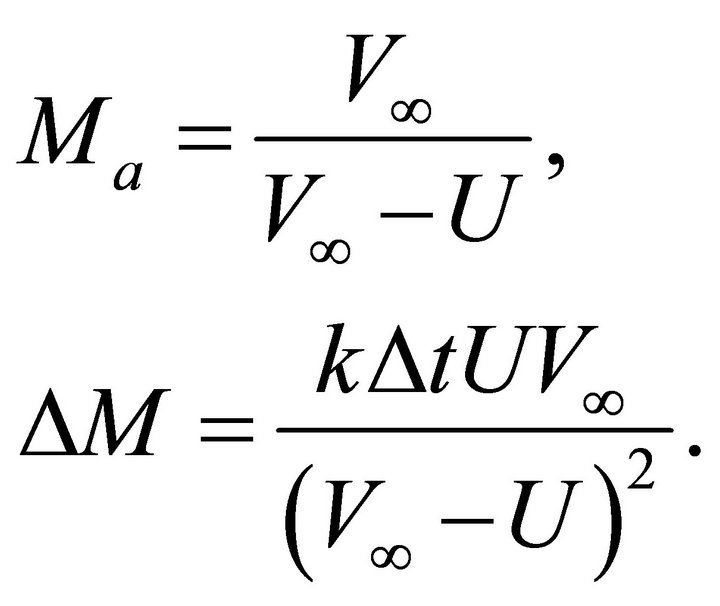
To simplify the equations for velocity transforms, it is suitable to introduce a special parameter M. This parameter can be defined at any point of the profile, and in particular, at the top and the bottom interfaces of an interval,
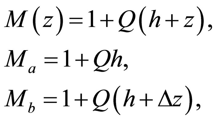 (25)
(25)
where  is the interval thickness (the vertical distance between the two interfaces), subscript a is related to the top interface
 , and subscript b is related to the bottom interface
 . It follows from Equation (25) that
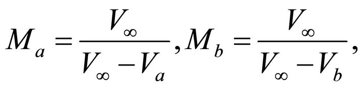 (26)
(26)
where  and
and  are the top and bottom instantaneous velocities, respectively. Next, it follows from Equation (26) that parameter M is the inverse normalized measure of the difference between the velocity at the given depth level and the asymptotic velocity
 . Equation (26) can be inverted,
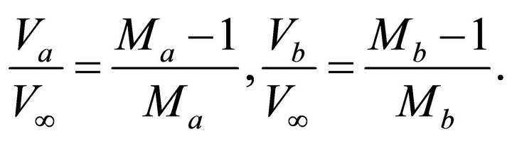 (27)
(27)
The velocity gradient is also related to the asymptotic factor,
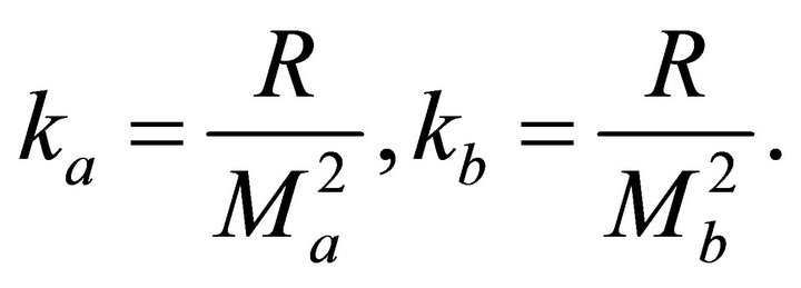 (28)
(28)
It follows from Equation (25) that
 (29)
(29)
and
 (30)
(30)
We use Equations (28) and (29) to get the interface gradients,  and
and , through the increment of the asymptotic factor,
  ,
,
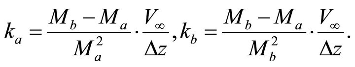 (31)
(31)
It follows from Equation (31),
 (32)
(32)
Equations (27) and (29) result in the average gradient on the interval,  , expressed either through the interface asymptotic factors
  and
and , or through the interface gradients
  and
and ,
,
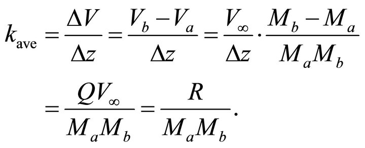 (33)
(33)
Introduction of Equation (28) into Equation (33) leads to
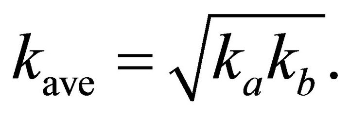 (34)
(34)
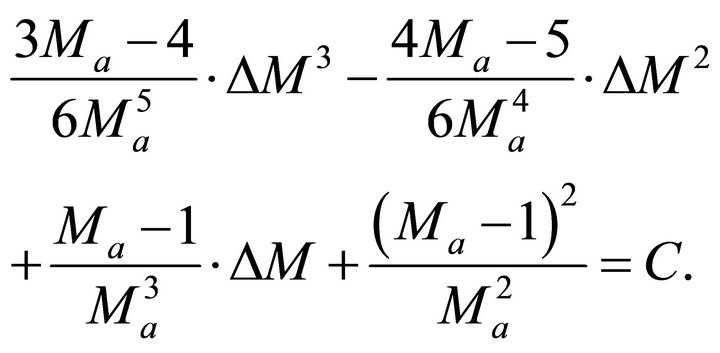
The average gradient on the interval with the Hyperbolic velocity profile is the geometric average of the top and bottom interface gradients.
Given the velocity and its gradient at one interface, one can calculate these parameters at the other interface. The calculations can be done either in depth or in time. Four problems of this kind are considered in Appendix C.
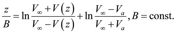
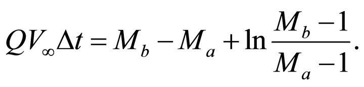
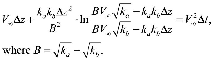
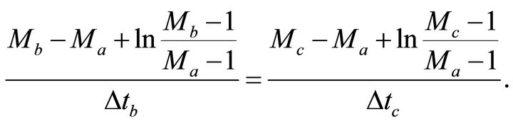
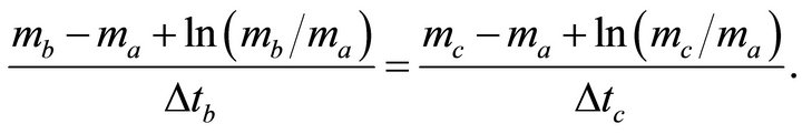
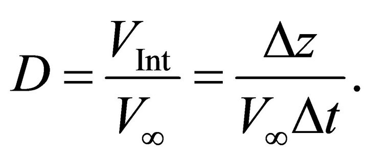
4. Depth-Traveltime Relationship
Integrate the slowness to get the vertical traveltime vs. the interval thickness,
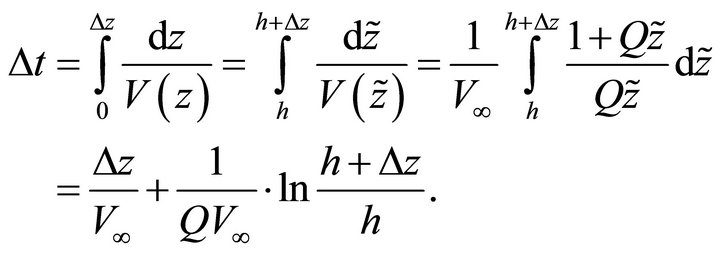 (35)
(35)
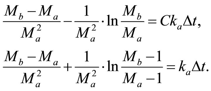
The traveltime equation can be written in terms of asymptotic factors at the top and bottom interfaces,  and
and . With the use of Equations (25) and (29), we obtain
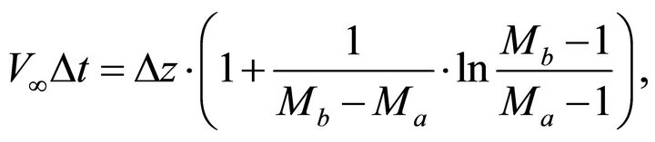 (36)
(36)
where the top asymptotic factor  is calculated with Equation (26), and the bottom asymptotic factor
  - with the first equation of Equation Set (32). The interval velocity (local average velocity) through the layer between the interfaces becomes
 (37)
(37)
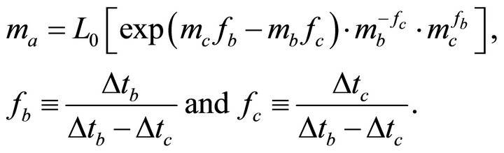
To get the vertical distance vs. traveltime we should invert Equation (26), i.e. find . Introduction of Equation (29) into (36) results in
 (38)
(38)
Equation (38) should be solved for the unknown bottom asymptotic factor ,
,
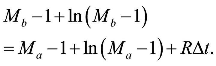 (39)
(39)
Taking exponent from both sides of Equation (39), we get
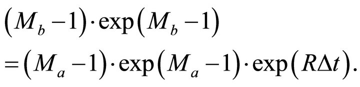 (40)
(40)
Equation (40) can be solved with the Lambert function,
 (41)
(41)
where notation  means the zero branch of the Lambert function. The Lambert function
 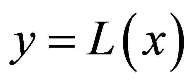 delivers the solution of the transcendent equation
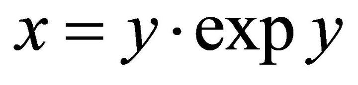 , see Appendix B for details. In terms of the interface velocities, Equation (41) reduces to
 (42)
(42)
After the bottom asymptotic factor  or the bottom interface velocity
  is found, the interval thickness can be established with Equation (29),
 (43)
(43)
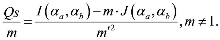
5. Hyperbolic and Non-Hyperbolic Moveout
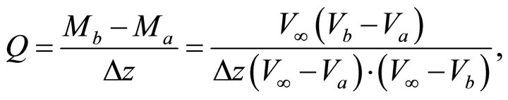
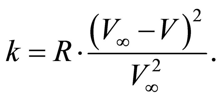
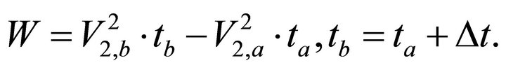
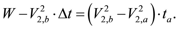
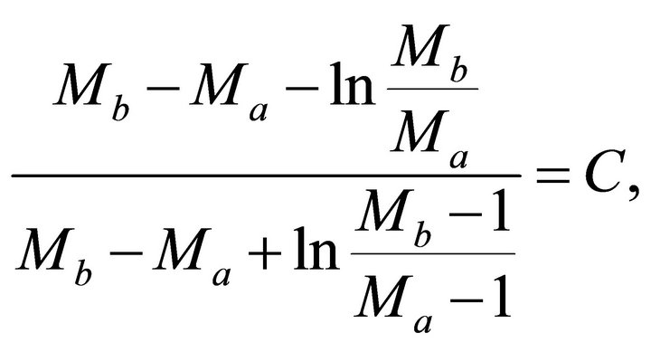
In the absence of the intrinsic anellipticity, the hyperbolic parameter W and the non-hyperbolic parameter H on the interval are defined as
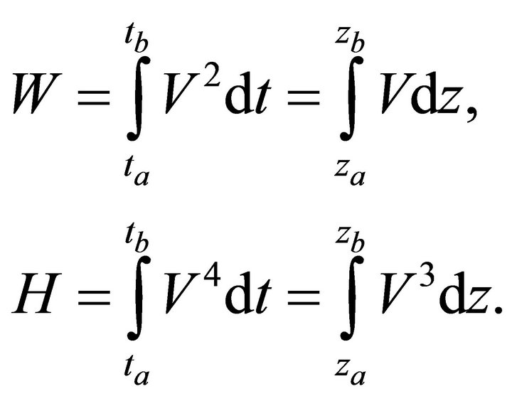 (44)
(44)
Introduce the velocity profile from Equation (17). The hyperbolic parameter W becomes
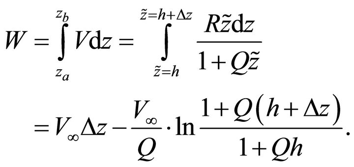 (45)
(45)
The non-hyperbolic parameter H becomes
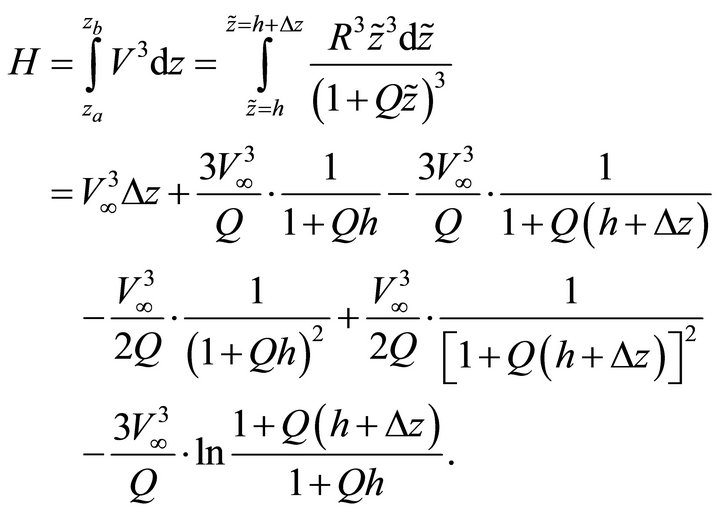 (46)
(46)
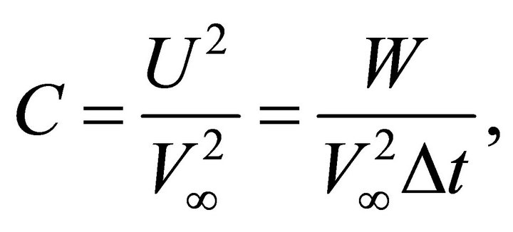
With the use of the top and bottom asymptotic factors, the hyperbolic parameter becomes
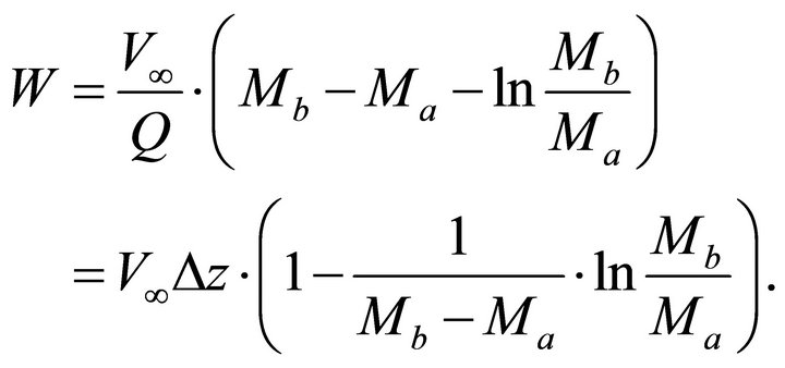 (47)
(47)
Introducing Equation (37) for the traveltime into Equation (47), we obtain the local RMS velocity U over the interval. By definition, 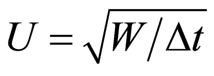 , so
, so
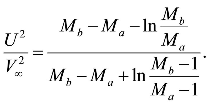 (48)
(48)
The non-hyperbolic parameter becomes
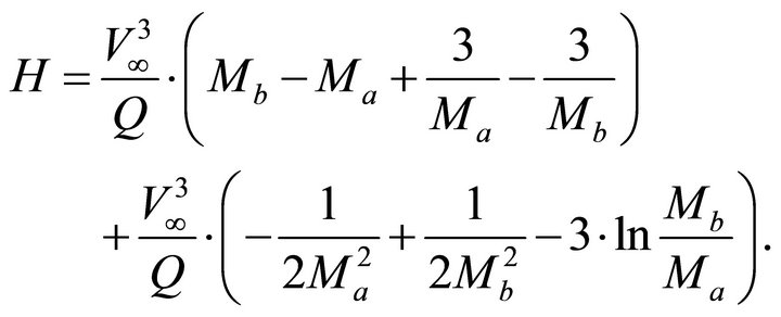 (49)
(49)
With the use of Equation (29), the non-hyperbolic parameter simplifies to
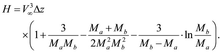 (50)
(50)
When the parameters of the velocity profile are specified, the top asymptotic factor Ma is a known value. The bottom asymptotic factor Mb can be presented either vs. depth (interval thickness) or vs. traveltime. Thus, the hyperbolic and non-hyperbolic parameters become functions of depth or traveltime, accordingly. The anellipticity induced by the vertically varying velocity is defined as the fractional difference between the fourth-order average velocity  and the RMS velocity
 ,
,
 (51)
(51)
Parameter  can be also considered as a function of depth or vertical time. For a particular case of a single infinite layer (half-space) with any vertical velocity profile,
 (52)
(52)
The graph for the induced anellipticity  is plotted vs. depth in Figure 3 for three asymptotically bounded velocity models: Exponential, Conic and Hyperbolic. For all the three models, the parameters of the velocity profile are:
 and
and . At the surface, the anellipticity is zero as there are yet no accumulated variations of the instantaneous velocity. The induced anellipticity is always positive. It reaches a maximum value a definite depth and then vanishes at the
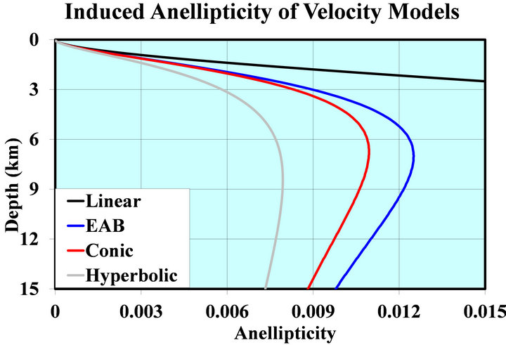
Figure 3. Induced anellipticity vs. depth for asymptotically bounded velocity models.
infinity, where the medium velocity is asymptotically constant.
6. Forward Dix Transform
Consider a package of n layers (vertical intervals), where the nodes (interfaces) are enumerated from zero, and layers are enumerated from 1. Interval n connects nodes  (top interface) and n (bottom interface). The nodal average velocity
 , RMS velocity
  and fourthorder average velocity
  are
are
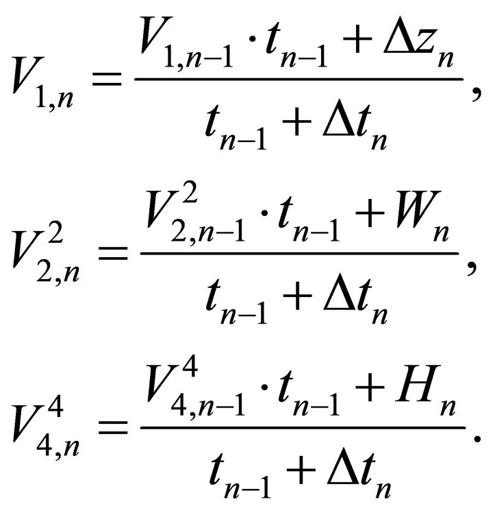 (53)
(53)
where  is the one-way interval traveltime,
 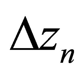 is the layer thickness, Wn and Hn are the interval hyperbolic and non-hyperbolic parameters, respectively. For
 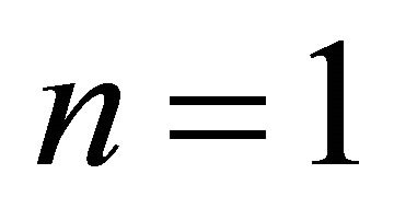 we set
  in Equation (53). The effective velocities (average, RMS and fourth-order average) can be also defined for any internal point of the interval.
7. Inverse Dix Transform
Recall that the Hyperbolic velocity profile on the interval is defined by the three parameters: the top interface instantaneous velocity , the top interface gradient
 , and the asymptotic velocity
 . We consider that the asymptotic velocity is always given a priori. When the two other parameters,
  and
and , are also known, then velocity transforms are considered forward. When one or both parameters are unknown (with another data specified instead), we deal with the velocity inversion. There are three groups of inverse transforms studied in Appendices D, E and F.
Appendix D considers the inversion that does not involve the RMS velocity. These formulations deal with the instantaneous velocity and its gradient only. We solve a problem where the two velocities are given at the interfaces,  and
and , or—alternatively—the two gradients,
  and
and . Another kind of problem is when the velocity and its gradient are given at the different interfaces of the interval, i.e. the velocity is given at the top interface and the gradient—at the bottom interface,
  and
and , or vice versa,
  and
and . We solve also a problem where the instantaneous velocity is given at the bottom interface and at the intermediate point of the interval,
  and
and . These problems are studied both vs. depth and vs. time.
Appendix E considers the inversion with the RMS velocity specified at the interfaces vs. depth or time with a single parameter unknown, either  or
or . We consider also a problem with the traveltime specified vs. the interval thickness, also with a single parameter unknown. Finally, we consider the RMS velocity specified vs. both depth and time, with the two parameters unknown,
  and
and .
.
In Appendix F we study the two-interval inversion. The RMS velocity is given vs. depth or time at the two interfaces and at an internal point of the interval. Alternatively, depth can be specified vs. traveltime at the three points. Both parameters of the velocity profile are unknown. This is a so-called three-point or two-interval inversion.
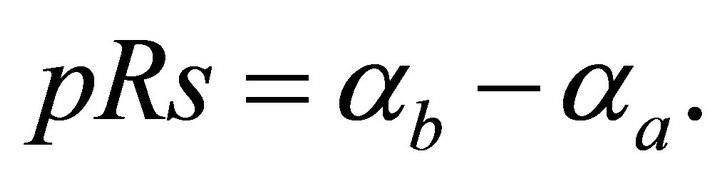
8. Ray Trajectories
In this section we establish the trajectories of non-vertical rays. Due to Snell’s law, in 1D medium the horizontal slowness ![]() is constant, and the ray angle
is constant, and the ray angle ![]() (measured from the vertical axis) becomes
(measured from the vertical axis) becomes
 (54)
(54)
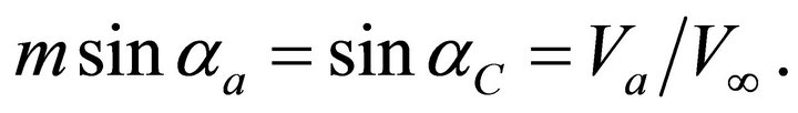
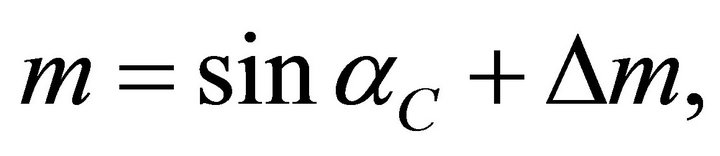
Introduce the ray parameter m,
 (55)
(55)
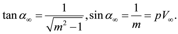
where Q and R are the physical parameters of the Hyperbolic velocity profile,  is the normalized ray slowness, and m is its inverse value. We call parameter m “eccentricity of the ray trajectory” as it is very similar to the eccentricity of the hyperbolic and elliptic rays of the Conic velocity model [13]. With Equation (17), the sine of the ray angle becomes
 (56)
(56)
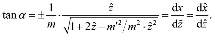
so that the tangent of this angle is
 (57)
(57)
where . Parameter
  (the conjugate eccentricity squared) may be positive or negative. Introduce the dimensionless coordinates,
 (58)
(58)
The tangent of the ray angle becomes
 (59)
(59)
Integrating Equation (59), we obtain
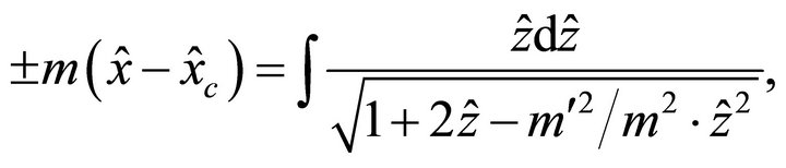 (60)
(60)
where  is the constant of integration. This integral can be reduced to
 (61)
(61)
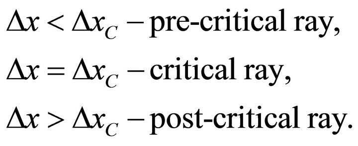
To obtain the integral on the right side of Equation (61), we consider two cases, or two ranges of the eccentricity: m > 1 (pre-critical rays) and m < 1 (post-critical rays),
 (62)
(62)
For a limiting case  (critical rays),
 (63)
(63)
We emphasize that two kinds of rays exist for any monotonously increasing and asymptotically bounded velocity model, and in particular, for the Hyperbolic model. The pre-critical rays that may start on the earth surface, propagate to the infinite depth, and their curvature asymptotically vanishes. The post-critical rays have a limited propagation depth. Their arc-like trajectories have a finite minimum curvature at the turning point, and these rays return to the earth surface. Note that at any point of the trajectory, the ray path curvature  depends on the velocity gradient k only,
 (64)
(64)
In particular, the linear velocity model with a constant velocity gradient leads to ray trajectories of constant curvatures, i.e. to the circular arcs.
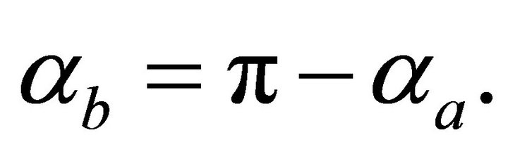
The critical rays with the unit eccentricity  are the limit case between the two types of rays. Their takeoff angle (the ray angle at the upper interface) is called the critical angle
 . It follows from Equations (54) and (55) that the critical take-off angle is
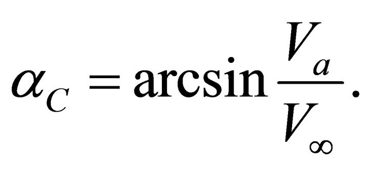 (65)
(65)
It follows from Equations (61) and (62) that the trajectories of the pre-critical and post-critical rays are
 (66)
(66)
At infinite depth, pre-critical rays become asymptotically straight. Equation (57) leads to
 (67)
(67)
However, although the slope of these rays converges to a constant value and their curvature becomes infinitesimal, the pre-critical rays of the Hyperbolic model have no asymptotic straight line, unlike the pre-critical rays of the EAB and the Conic models. The pre-critical, critical and post-critical rays are plotted in Figure 4 for the Hyperbolic, the Conic and the Exponential (EAB) models. Parameters of the velocity profile are the same
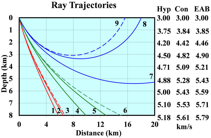
Figure 4. Pre-critical (red lines), critical (green lines) and post-critical (blue lines) ray trajectories for Hyperbolic (lines 1, 4, 7), Conic (lines 2, 5, 8) and EAB (lines 3, 6, 9) velocity models. Pre-critical rays propagate to an infinite depth and become asymptotically straight. Critical ray propagate to an infinite depth, and the ray angle approaches π/2 at large depth, but this ray has no asymptote. Postcritical rays pass the turning point and return to the earth surface, their trajectories are symmetric arcs. The Conic rays pass above the Hyperbolic model rays because their curvature is larger. For the same reason, the EAB rays pass above the Conic rays. For all models, parameters of the medium are the same as in Figure 1. The take-off angle of the pre-critical rays is 3π/24, that of the critical rays π/6, and that of the post-critical rays 5π/24.
as above. The three columns of numbers to the right of the plot area are velocities for the three models at the specified depth levels.
9. Maximum Penetration Depth
Pre-critical rays penetrate to infinite depth. The maximum penetration depth of post-critical rays follows from Equation (59). At the turning point, the ray angle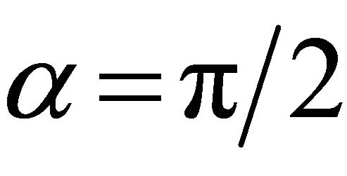 , and thus, its tangent becomes infinite. This leads to a quadratic equation with a single positive root,
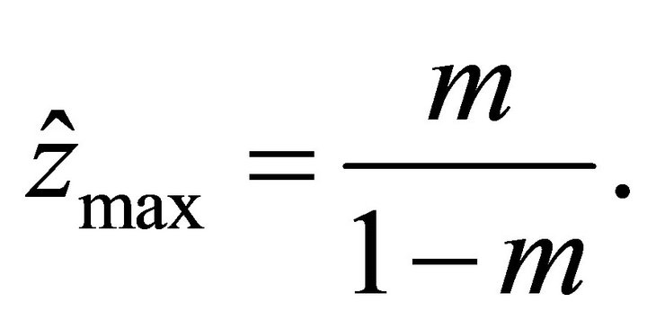 (68)
(68)
Recall that  is the dimensionless depth measured from the absolute origin (above the upper interface). The maximum penetration depth in units of length, measured from the upper interface reads
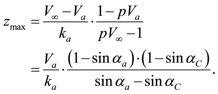 (69)
(69)
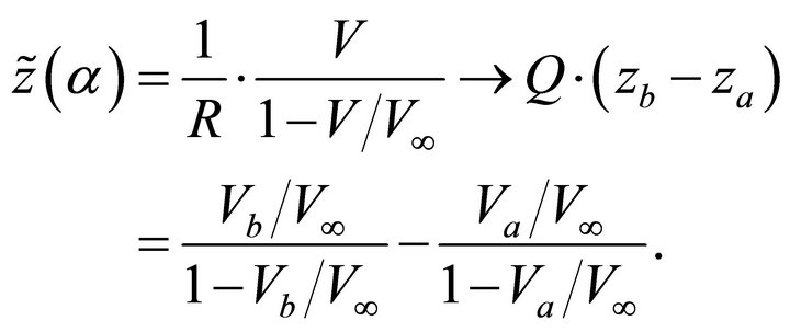
10. Lateral Propagation, Traveltime and Arc Length
In a 1D medium, it is convenient to express the lateral propagation distance![]() , traveltime
, traveltime ![]() and arc length
and arc length ![]() through the ray angle
through the ray angle ![]() and angle-dependent gradient
and angle-dependent gradient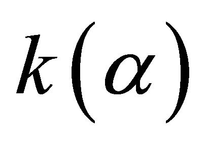 . These relationships are [12,16] (Kaufman, 1953; Ravve and Koren, 2006)
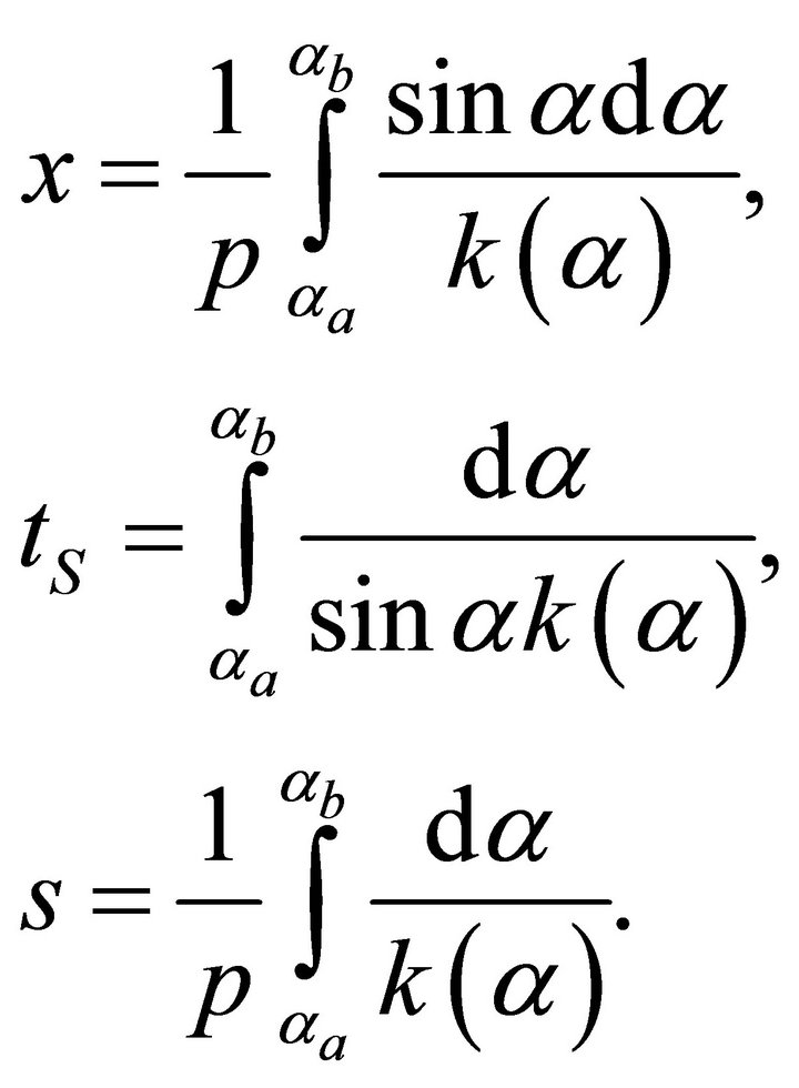 (70)
(70)
where  and
and  are ray angles at the departure and the destination points, respectively. Equations (17) and (19) make it possible to eliminate depth and to express the gradient through the velocity,
 (71)
(71)
Next we apply Snell’s law and obtain the vertical gradient vs. the ray angle,
 (72)
(72)
Note that
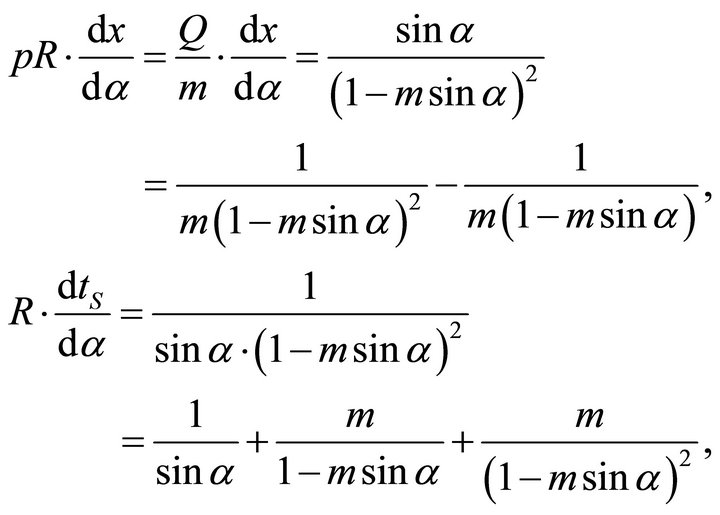 (73)
(73)
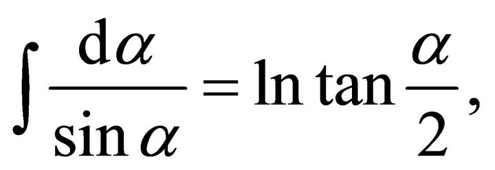 (74)
(74)
 (75)
(75)
The indefinite integral on the right side of this equation essentially depends on the range of the eccentricity m, resulting in
 (76)
(76)
For the critical ray, 
 (77)
(77)
Let  and
and  be the ray angles at the start point and the destination point of the ray path, respectively. Equation Set (76) can be re-arranged as follows
• For the pre-critical rays, 
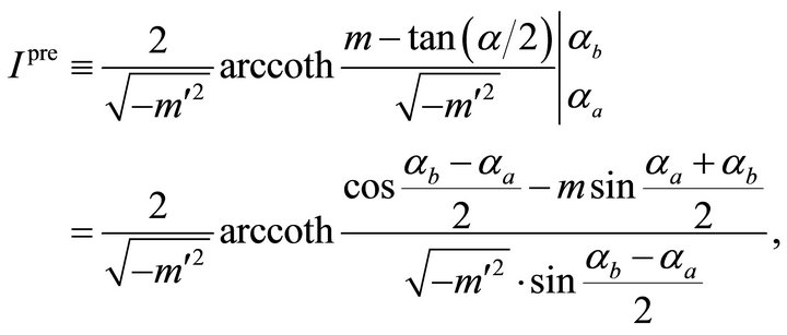 (78)
(78)
• For the post-critical rays, 
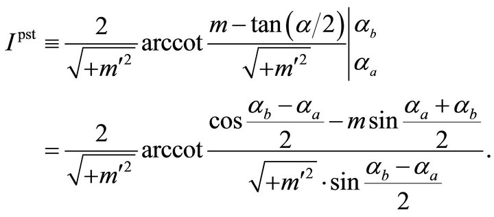 (79)
(79)
 and
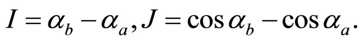
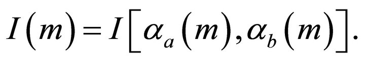
and  are functions of the ray angles at the endpoints of the path. The following identities were used,
 (80)
(80)
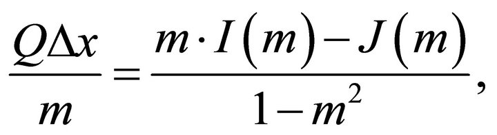
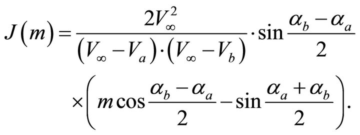
To simplify the notations, we introduce one more function of the ray angles at the endpoints,
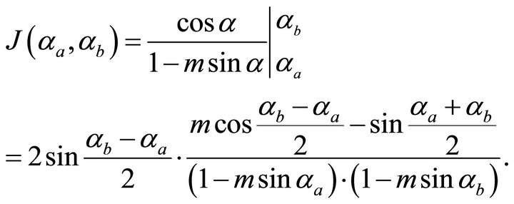 (81)
(81)
The normalized lateral propagation becomes
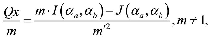 (82)
(82)
The normalized traveltime is
 (83)
(83)
The normalized arc length is
 (84)
(84)
For the critical rays,  , and the departure angle is critical,
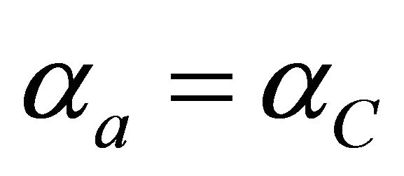 . The ray path parameters are,
 (85)
(85)
The current depth can be also expressed through the ray angle. It follows from Equation (17) that
 (86)
(86)
Recall that
 (87)
(87)
and therefore
 (88)
(88)
In Figure 5 we plot the graphs for the traveltime vs. ray path arc length for the pre-critical, the critical and the post-critical rays of the Hyperbolic velocity profile.
The “trigonometric” solution for the lateral propagation and traveltime of the post-critical rays was obtained (in a different form) by Muscat (1937). However, it was not pointed out in this early study that the solution was related to the post-critical rays only, and that the other, “hyperbolic” solution exists for the pre-critical rays (and a “transient” solution for the critical rays, which are the limit case between the two basic types of rays).
Note that for the vanishing or infinitesimal parameter , the shape of the trajectory, the lateral propagation, the traveltime and the arc length of the Hyperbolic model ray path converge to the corresponding character-
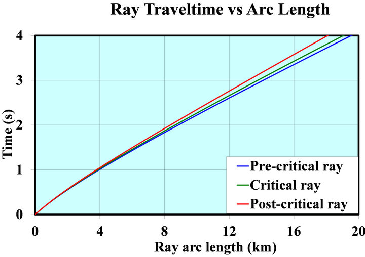
Figure 5. Traveltime vs. arc length of ray path for the three kinds of rays of the Hyperbolic velocity model: the precritical ray αa = 22.5˚, the critical ray αa = αC = 30˚ and the post-critical ray αa = 37.5˚.
istics of the linear velocity profile. In this case the asymptotic velocity  becomes unbounded, so that the product
 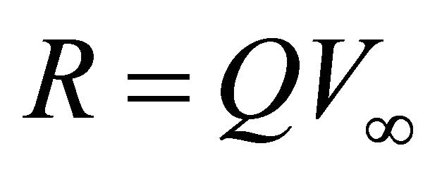 remains a finite value and converges to a constant gradient of the linear velocity model. The eccentricity m becomes infinitesimal, and
 (89)
(89)
Functions I and J from Equations (79) and (81) simplify to
 (90)
(90)
Equation (66) comes to
 (91)
(91)
This is an equation for the circular arc of radius 
whose center is located at  where
where ![]() is the ray slowness. The lateral propagation, Equation (82), becomes
is the ray slowness. The lateral propagation, Equation (82), becomes
 (92)
(92)
Equation (83) yields the traveltime for this limiting case,
 (93)
(93)
and finally, Equation (84) for the arc length converges to
 (94)
(94)
11. Full Arc of Post-Critical Ray
Consider two points on the earth surface, the transmitter and the receiver, located  distance apart. The goal is to trace the full arc of the post critical turning ray that connects the two points. Note that due to the symmetry of the arc, the ray angle at the destination point
  is related to the take-off angle
  ,
,
 (95)
(95)
Applying Equations (79), (81) and (82), we obtain
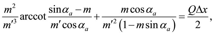 (96)
(96)
where 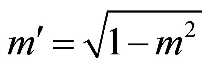 is the conjugate eccentricity of the post-critical ray path. Recall that
 (97)
(97)
Equation (96) simplifies to
 (98)
(98)
Equation (98) should be solved numerically for the unknown eccentricity m. To obtain the initial guess, we assume that the distance  is small. Then the take-off angle
  approaches
 , and according to Equation (97), the eccentricity exceeds the sine of the critical angle only slightly. We assume
 (99)
(99)
where  is a small positive value. Next we expand Equation (98) into the Taylor series and neglect the high order terms,
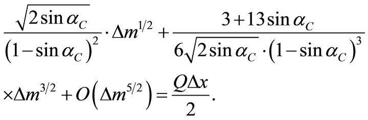 (100)
(100)
The cubic Equation (100) has a single positive root. For example, for the velocity profile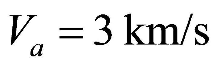 ,
,  and
and , and the offset
 , the critical angle becomes
 . Equation (100) leads to
 , and Equation (99) yields the initial guess
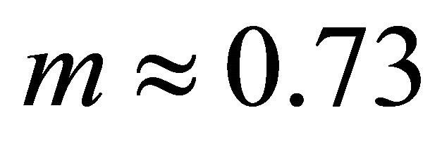 . Solving Equation (98) with the Newton method, we obtain the eccentricity
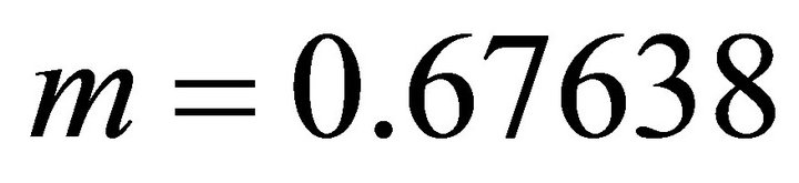 . The take-off angle becomes
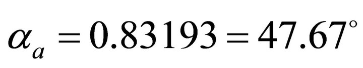 . The arcs are plotted in Figure 6 for the three asymptotically bounded velocity models. In the shallow region, the Hyperbolic model has a smaller vertical gradient (and thus, a smaller curvature) than the Conic and the EAB models, and thus, the Hyperbolic model yields a smaller take-off angle. The ray path arc of the Hyperbolic model passes above the Conic and the EAB arcs.
12. Boundary Value Ray Tracing
Given data are the departure point  and the arrival point
 , and the goal is to trace the ray path. The ray path is an explicit function of the eccentricity m, and this parameter is so far unknown. Without any loss of generality, we assume here that
 , i.e. that the lateral distance
  and the horizontal ray slowness
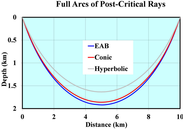
Figure 6. Full arcs of post-critical rays for the EAB, the Conic and the Hyperbolic velocity profiles.
p are positive. Assume also , which is also not a limitation (one can reverse the endpoints otherwise). Since the ray tracing equations depend on the type of ray, we need to determine, whether the ray is pre-critical or post-critical. For this, one can plot a critical path that starts at the departure point at the critical take-off angle
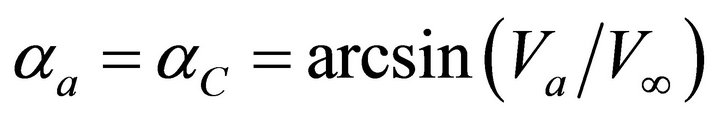 . If the destination point lays to the left from the critical trajectory, then the ray path is pre-critical. The ray path is post-critical if the destination point lays to the right. The critical lateral propagation
  is delivered by Equation (63), which can be rearranged as
 (101)
(101)
Given the vertical coordinates of the source and the receiver,  and
and , we calculate the critical lateral propagation, and then apply the criterion
 (102)
(102)
The velocities at the end points of the trajectory  and
and  are known values. It follows from Snell’s law that the ray angles at the end points of the trajectory are the functions of the eccentricity alone,
 (103)
(103)
Note that for the pre-critical rays and for the post critical rays before the turning point, the ray angle is acute, while for the turning rays after the turning point the ray angle is obtuse,
 (104)
(104)
Equation (82) relates the lateral propagation  to the ray angles at the endpoints, which, in turn, depend on the eccentricity according to Equations (103) and (104),
 (105)
(105)
where
 (106)
(106)
Function
 (107)
(107)
is delivered by Equations (78) and (79). It was initially defined as a function of the endpoints’ ray angles, but due to Equations (103) and (104) it can be considered as a function of the eccentricity alone. Next we solve nonlinear Equation (105) numerically for the unknown eccentricity m. Then the ray angles at the endpoints can be established, and the ray path can be plotted with Equation (66). Numerical examples for the boundary value ray tracing with the Hyperbolic velocity profile are presented in Appendix G.
13. Conclusion
The Hyperbolic asymptotically bounded exponential velocity model has been studied and compared to other asymptotically bounded models, in particular, the Exponential and the Conic. The forward and the inverse velocity transforms are derived. The Hyperbolic model allows a better representation of the vertical velocity variations in compacted sediments, especially in the case of thick layers. An advantage of the Hyperbolic model is that the instantaneous velocity reaches the asymptotic value in a more slow and gradual fashion, as compared to other asymptotically bounded models. Ray tracing equations have been derived. The ray trajectories, traveltimes and arc lengths have been studied analytically, and the boundary value ray tracing problem have been solved. We have tried to present a complete theory for both vertical and non-vertical rays propagating through the Hyperbolic model. Application of the Hyperbolic velocity distribution enables us to present realistic geological models using fewer parameters, as compared to the classical linear velocity function. We showed that the linear velocity function is a limiting particular case of the Hyperbolic model.
14. Acknowledgements
We are grateful to Paradigm Geophysical for the financial and technical support of this study and for the permission to publish its results.
REFERENCES
- M. Muskat, “A Note on Propagation of Seismic Waves,” Geophysics, Vol. 2, No. 4, 1937, pp. 319-328. doi:10.1190/1.1438098
- M. M. Slotnick, “On Seismic Computations, with Applications, Part I,” Geophysics, Vol. 1, No. 1, 1936, pp. 9-22. doi:10.1190/1.1437084
- M. M. Slotnick, “Lessons in Seismic Computing,” Society of Exploration Geophysicists, Oklahoma, 1959.
- M. M. Slotnick, “On Seismic Computations, with Applications, Part II,” Geophysics, Vol. 1, No. 3, 1936, pp. 299-305. doi:10.1190/1.1437111
- M. Al-Chalabi, “Instantaneous Slowness versus Depth Functions,” Geophysics, Vol. 62, No. 1, 1997, pp. 270- 273. doi:10.1190/1.1444127
- C. H. Chapman and H. Keers, “Application of the Maslov Seismogram Method in Three Dimensions,” Studia Geophysica et Geodaetica, Vol. 46, No. 4, 2002, pp. 615-649. doi:10.1023/A:1021104820892
- C. E. Houston, “Seismic Paths, Assuming a Parabolic Increase of Velocity with Depth,” Geophysics, Vol. 4, No. 4, 1939, pp. 232-236. doi:10.1190/1.1440500
- M. Al-Chalabi, “Parameter Non-Uniqueness in Velocity versus Depth Functions,” Geophysics, Vol. 62, No. 3, 1997, pp. 970-979. doi:10.1190/1.1444203
- L. Y. Faust, “Seismic Velocity as a Function of Depth and Geologic Time,” Geophysics, Vol. 16, No. 2, 1951, pp. 192-206. doi:10.1190/1.1437658
- L. Y. Faust, “A Velocity Function Including Lithologic Variation,” Geophysics, Vol. 18, No. 2, 1953, pp. 271- 288. doi:10.1190/1.1437869
- I. Ravve and Z. Koren, “Exponential Asymptotically Bounded Velocity Model, Part I: Effective Models and Velocity Transformations,” Geophysics, Vol. 71, No. 3, 2006, pp. T53-T65. doi:10.1190/1.2196033
- I. Ravve and Z. Koren, “Exponential Asymptotically Bounded Velocity Model, Part II: Ray Tracing,” Geophysics, Vol. 71, No. 3, 2006, pp. T67-T85. doi:10.1190/1.2194897
- I. Ravve and Z. Koren, “Conic Velocity Model,” Geophysics, Vol. 72, No. 3, 2007, pp. U31-U46. doi:10.1190/1.2710205
- Z. Koren and I. Ravve, “Constrained Dix Inversion,” Geophysics, Vol. 71, No. 6, 2006, pp. R113-R130. doi:10.1190/1.2348763
- E. Robein, “Velocities, Time-Imaging and Depth-Imaging in Reflection Seismics: Principles and Methods,” EAGE Publications, Houten, the Netherlands, 2003.
- H. Kaufman, “Velocity Functions in Seismic Prospecting,” Geophysics, Vol. 18, No. 2, 1953, pp. 289-297. doi:10.1190/1.1437871
- R. M. Corless, G. H. Gonnet, D. G. Hare, D. J. Jeffrey and D. D. Knuth, “On the Lambert W Function,” Advances in Computational Mathematics, Vol. 5, No. 1, 1996, pp. 329-359. doi:10.1007/BF02124750
Appendix A. Gradient-Velocity Diagrams
In this appendix we derive the gradient-velocity diagrams for the five asymptotically bounded velocity models. In all cases we pass to a shifted frame , in which the governing equations are essentially simplified. The value of the vertical shift h is different for all models. For all models the “absolute” origin corresponds to a point of maximum gradient. For all models except the Exponential slowness, this is also the point of a vanishing instantaneous velocity. As we show below, for the Exponential slowness model, the absolute origin corresponds to the half-limiting velocity
 .
.
A.1. The Hyperbolic Muscat Model
The velocity profile is given by
 (A-1)
(A-1)
Establish the depth level where the velocity vanishes. This point is located above the earth surface,
 (A-2)
(A-2)
Introduce the shifted frame, . The velocity profile becomes
 (A-3)
(A-3)
The vertical gradient is
 (A-4)
(A-4)
At the absolute origin , the gradient is maximal,
 (A-5)
(A-5)
Introduction of Equation (A-5) into (A-3) and (A-4) leads to
 (A-6)
(A-6)
Finally, elimination of depth  from the two equations of Equation Set (A-6) results in
 (A-7)
(A-7)
A.2. The Exponential Muscat Model
The velocity model is described by
 (A-8)
(A-8)
The vertical shift is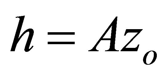 , and in the shifted frame,
 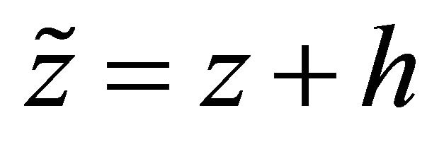 , Equation (A-8) simplifies to
 (A-9)
(A-9)
The velocity gradient is
 (A-10)
with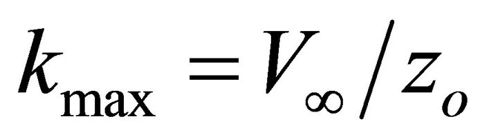 , so that
 (A-11)
Eliminate the absolute depth from Equations (A-9) and (A-11) and obtain the gradient-velocity relationship,
 (A-12)
A.3. The Exponential Slowness Model
The profile equation reads
 (A-13)
Unlike the other asymptotically bounded models mentioned in the introduction, the velocity in the Exponential slowness model does not vanish at a finite negative depth. The velocity vanishes at ![]() and approaches to the asymptotic value
and approaches to the asymptotic value  at
at . The gradient of the velocity is
 (A-14)
The gradient  vanishes at both remote ends,
 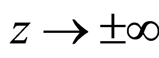 , and
, and  has a single critical point: the maximum of the gradient occurs at
 ,
,
 (A-15)
We emphasize that the logarithm in Equation (A-15) may prove to be both positive and negative. At the point , the maximum gradient and the velocity are
 (A-16)
Note that in case when the depth of the maximum gradient is positive,  , this point really exists underground, and the gradient first increases, then accepts the maximum value
 (A-17)
Below this point, the gradient begins to decay, and eventually vanishes at the infinite depth. In case when the depth  of the maximum gradient is negative, this point is above the earth surface, and throughout the whole depth range
  the velocity gradient
  is actually a monotonously decreasing function. Note that
 (A-18)
Next we assume the shift , and pass to the shifted frame,
 . The gradient accepts now a maximum value at the origin. Rearrange Equation (A- 13),
 (A-19)
Note that the velocity profile in Equation (A-19) can be set in an alternative way,
 (A-20)
where
 (A-21)
so that
 (A-22)
Finally, we eliminate depth from Equation (A-22) and obtain
 (A-23)
A.4. The Exponential Asymptotically Bounded Velocity Model (EAB)
In this case the velocity profile is
 (A-23)
The velocity vanishes above the earth surface at ,
,
 (A-24)
In the shifted frame , the velocity profile simplifies to
 (A-25)
At the shifted origin the gradient is maximal,
 (A-26)
Introduce Equation (A-26) into (A-25),
 (A-27)
Finally, we eliminate depth from Equation (A-27) and obtain the governing equation,
 (A-28)
Note that only for the EAB velocity model the diagram Equation (A-28) is linear.
A.5. Conic Velocity Model
For the Conic profile, the velocity and its gradient in the absolute frame are given by
 (A-29)
This equation can be rearranged as
 (A-30)
Next we eliminate the absolute depth  from Equation (A-29) and get the governing differential equation of the Conic velocity model,
 (A-31)
The Conic velocity profile, Equation (A-30), can be also set in an equivalent form, through a hyperbolic and an inverse hyperbolic function,
 (A-32)
A.6. Comments on Diagrams
Summarize the gradient-velocity diagrams for the five asymptotically bounded velocity models. The governing differential equations are
 (A-33)
The gradient-velocity diagrams for the five asymptotically bounded models are plotted in Figure 7. Note that in the original frame of reference the asymptotically bounded models are described by the three parameters. As we mentioned, in the shifted frame where the velocity vanishes at the origin (or the vertical gradient accepts a maximum value at the origin), only two parameters are needed. These two parameters may be the maximum gradient  and the asymptotic velocity
  as in Equation Set (A-33). The constant value that appears upon the integration of each equation is not a new parameter as it should be adjusted to match the maximum values
  and
and .
.
We emphasize that only for the EAB model the gradient-velocity relationship is linear: Derivative of an exponent is proportional to the same exponent.
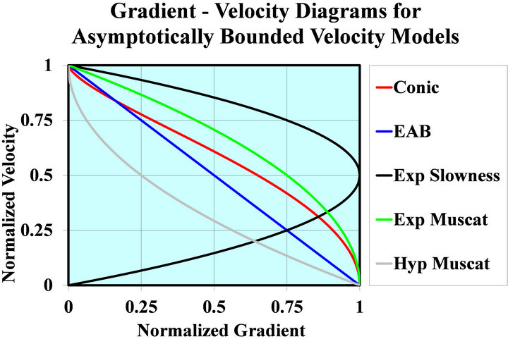
Figure 7. Diagrams “Gradient-Velocity” for asymptotically bounded velocity models. Only for the EAB model the diagram is linear. For all models, except the Exponential slowness model, the gradient decreases with the increase of velocity. For the Exponential slowness model the gradient reaches maximum when the velocity becomes one half of the asymptotic value. Note the central symmetry between the two Muscat models, Hyperbolic and Exponential.
For all models except the Exponential slowness [8], the gradient decreases with the increase of velocity (and depth). In case of the Exponential slowness, the vertical gradient increases along with the velocity, until the velocity reaches one half of the asymptotic value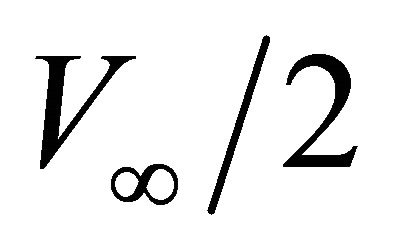 . At this point the gradient reaches its maximum value
 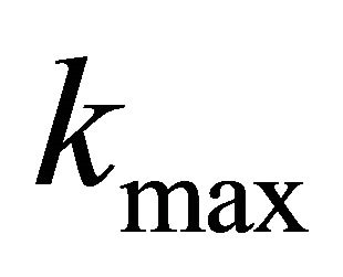 and then begins to decrease with depth. The point of maximum gradient in the Exponential slowness model may really exist in the subsurface, or it may be an imaginary point located above the earth surface (or above the upper interface of a layer). This point is real in case when the initial velocity
  does not exceed the halflimiting value,
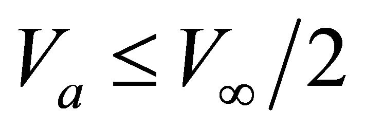 . Furthermore, we comment on the special central symmetry between the two Muscat (1937) models: Hyperbolic (HM) and Exponential (EM), see Equation (A-33) and the two corresponding plots in Figure 7,
 (A-34)
where ![]() and
and  are the corresponding gradientvelocity functions in Equation (A-33) for these two models. Although these two models are described by essentially different vertical velocity profiles, there is an apparent similarity in the gradient-velocity diagrams.
Appendix B. Lambert Function
The Lambert function [17]  delivers the solution of the transcendent equation
 (B-1)
(B-1)
Its graph is plotted in Figure 8 and consists of two branches: branch zero  and branch minus one
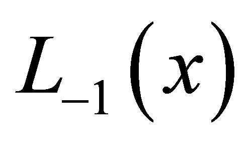 . The argument range is
  for branch zero and
  for branch minus one. The value range is
  for branch zero and
  for branch minus one. In particular, this
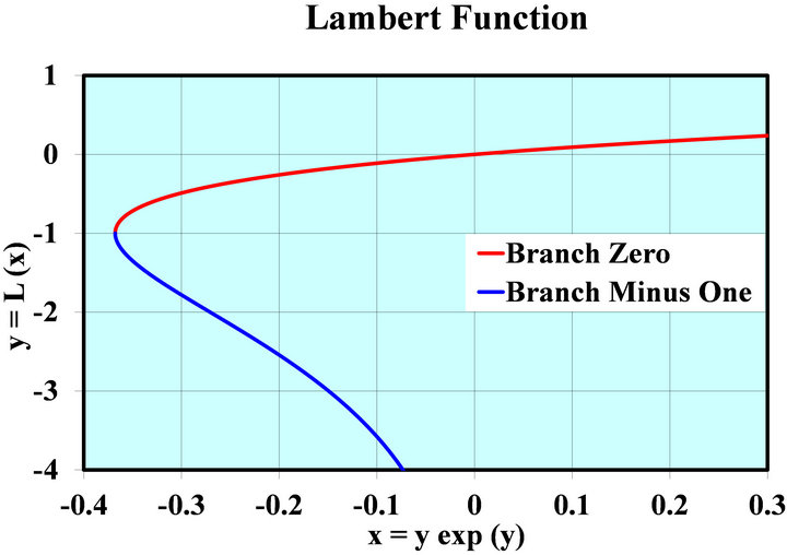
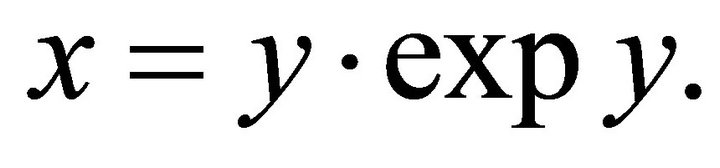
Figure 8. Lambert function y = L(x) is the solution of the transcendent equation y·exp(y) = x for a given value x and an unknown value y. The function has two branches. Branch zero is plotted in red, and branch minus one is plotted in blue.
means that for a positive argument x only branch zero exists, while for a negative argument both branches do exist. Therefore, in the latter case, the branch index should be specified to avoid ambiguity. The derivative of the Lambert function is
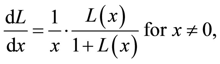 (B-2)
(B-2)
and for the infinitesimal argument
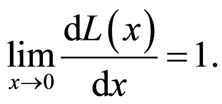 (B-3)
(B-3)
Comment. A general comment is related to Appendices C to F. The transform equations are formulated in the dimensionless form, with the unknown top and bottom asymptotic factors,  and
and . After the transform equation or equation set is resolved, we apply Equation (27) to find the top and bottom instantaneous velocities,
  and
and . If the transform is formulated in depth (i.e., the interval thickness
  is specified), we apply Equation (31) to find the top and bottom gradients of velocity,
  and
and . If the transform is formulated in time (i.e., the interval traveltime
  is specified), then we first apply Equation (37) to establish the interval thickness
 , and then Equation (31) to find the top and bottom gradients.
Appendix C. Swapping Interfaces
In this appendix, we find the instantaneous velocity and its gradient at the bottom interface, given these parameters at the top interface, and vice versa, and consider these problems both vs. depth and vs. time.
Problem C1. Given the velocity  and its gradient
  at the top interface and the layer thickness
 , one can establish the corresponding parameters at the bottom interface. For this, we calculate the top asymptotic factor
  with the first equation of Equation Set (26). The bottom asymptotic factor
  can be obtained with the first equation of Equation Set (32).
Problem C2. The instantaneous velocity and its gradient are specified at the bottom interface and the interval thickness  is given. Velocity and gradient should be found at the top interface. Thus, parameters
  are given, and parameters
  are to be found. In this case calculate the bottom asymptotic factor
  with the second equation of Equation Set (26) and apply the second equation of Equation Set (32) to get the top get
 .
.
Problem C3. The velocity and its gradient at the top interface,  and
and  are given, the interval traveltime
  is known, and the bottom interface parameters
  and
and  should be found. Combining the first equation of Equation Set (32) and Equation (36), we eliminate the interval thickness
  and obtain
 (C-1)
(C-1)
where the top asymptotic factor  is known from Equation (26). Equation (C-1) should be solved for the unknown bottom asymptotic factor
 . We use a cubic approximation for Equation (C-1) to get the initial guess, assuming the increment of the asymptotic factor
  is small,
 (C-2)
(C-2)
Problem C4. The velocity and its gradient are specified at the bottom interface, along with the interval traveltime, and the profile parameters should be found at the top interface. Thus, parameters  and
and  are given, while parameters
  and
and  are to be established. For this, we combine the second equation of Equation Set (32) and Equation (36),
 (C-3)
(C-3)
The bottom asymptotic factor  is known from Equation (26), and Equation (C-3) should be solved for the unknown top asymptotic factor
 . The initial guess for
  can be found from
 (C-4)
(C-4)
Appendix D. Inversion with Instantaneous Velocity
In this appendix we consider inversion problems that do not involve the effective models (average and RMS velocity). In this inversion group, one or both parameters at the top interface,  and
and  are unknown, with the other data given instead. The group includes four problems vs. depth (interval thickness) and four similar problems vs. interval traveltime.
Problem D1. Instantaneous velocities vs. depth. Given data are the top and bottom interface instantaneous velocities,  and
and , the asymptotic velocity
  and the interval thickness
 . Find the top interface gradient
 . Solution. Apply Equation (26) to calculate the top and bottom asymptotic factors,
  and
and .
.
Problem D2. Instantaneous velocities vs. time. Given data are the top and bottom interface instantaneous velocities,  and
and , the asymptotic velocity
  and the interval traveltime
 . Find the top interface gradient
 . Solution. Apply Equation (26) to calculate the top and bottom asymptotic factors,
  and
and .
.
Problem D3. Gradients vs. depth. Given data are the top and bottom interface vertical gradients,  and
and , the asymptotic velocity
  and the interval thickness
 . Find the top interface instantaneous velocity
 . Solution. Solve Equation Set (32) for the unknown asymptotic factors,
  and
and ,
,
 (D-1)
(D-1)
Problem D4. Gradients vs. time. Given data are the top and bottom interface vertical gradients,  and
and , the asymptotic velocity
  and the interval traveltime
 . Find the top interface instantaneous velocity
 . Solution. Introduce solution (D-1) into the traveltime Equation (36). This leads to a nonlinear equation vs. the unknown interval thickness
 (D-2)
(D-2)
Equation (D-2) should be solved numerically. It is suitable to normalize the gradients and the interval thickness,
 (D-3)
(D-3)
The normalized equation becomes
 (D-4)
(D-4)
To get an initial guess, we expand Equation (D-4) into a power series and obtain a cubic approximation,
 (D-5)
(D-5)
After the interval thickness is found, apply solution (D-1).
Problem D5. Velocity and gradient vs. depth at different interfaces. Given data are the top interface velocity , the bottom interface vertical gradient
 , the asymptotic velocity
  and the interval thickness
 . Find the top interface gradient
 . Solution. Apply Equation (26) to calculate the top asymptotic factor
 . Introduce the normalized bottom gradient,
 (D-6)
(D-6)
With this notation, the second equation of Equation Set (32) becomes
 (D-7)
(D-7)
Taking into account that for an interval of vanishing thickness  the top and bottom asymptotic factors coincide
 , one can establish the single physical root of the quadratic equation,
 (D-8)
(D-8)
Problem D6. Velocity and gradient vs. depth at different interfaces. Given data are the top interface gradient , the bottom interface instantaneous velocity
 , the asymptotic velocity
  and the interval thickness
 . Find the top interface velocity
 . Solution. Calculate the bottom asymptotic factor
  with equation 26. Normalize the top gradient,
 (D-9)
(D-9)
Get the top asymptotic factor
 (D-10)
Problem D7. Velocity and gradient vs. time at different interfaces. Given data are the top interface velocity , the bottom interface vertical gradient
 , the asymptotic velocity
  and the interval traveltime
 . Find the top interface gradient
 . Solution. Apply Equation (26) to calculate the top asymptotic factor
 . Then solve the nonlinear Equation (C-3) for the unknown bottom asymptotic factor
 . To get the initial guess, we assume
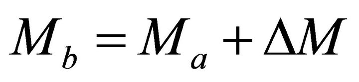 . Expand Equation (C-3) for a small increment of the asymptotic factor
 ![]() to get a cubic approximation,
to get a cubic approximation,
 (D-11)
Problem D8. Given data are the top interface gradient , the bottom interface instantaneous velocity
 , the asymptotic velocity
  and the interval traveltime
 . Find the top interface velocity
 . Solution. Apply Equation (26) to calculate the bottom asymptotic factor
 . To calculate the unknown top asymptotic factor, we solve the nonlinear Equation (C-1). To get the initial guess, assume
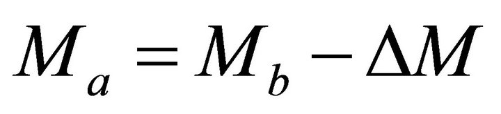 . This leads to
 (D-12)
Problem D9. Given data are the instantaneous velocity  at the bottom interface, and at an intermediate level inside the interval,
  , and the asymptotic velocity
 . Two vertical distances are specified: the full interval thickness
  (the distance between the top and bottom interfaces) and the partial interval thickness
  (the distance between the top interface and the intermediate level). Find the top interface velocity and gradient,
  and
and . Solution. Use Equation (26) to calculate the bottom asymptotic factor
  and the intermediate asymptotic factor
 . Apply Equation (29) for the full interval and for the partial interval,
 (D-13)
Solve Equation (D-13) for the top asymptotic factor ,
,
 (D-14)
Problem D10. Given data are the instantaneous velocity  at the bottom interface, and at an intermediate level
  inside the interval, and the asymptotic velocity
 . Two vertical traveltimes are specified: the full interval traveltime
  (the traveltime between the top and bottom interfaces) and the partial traveltime
  (the traveltime between the top interface and the intermediate level). Find the top interface velocity and gradient,
  and
and . Solution. Use Equation (26) to calculate the bottom asymptotic factor
  and the intermediate asymptotic factor
 . Apply Equation (28) for the full interval and for the partial interval, parameter
  becomes,
 (D-15)
Introduce parameter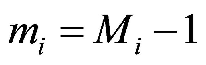 , Equation (D-15) becomes
 (D-16)
Equation (D-16) can be solved with the Lambert function, branch zero,
 (D-17)
Appendix E. Two-Point Effective Model Inversion
In this appendix we consider the two-point (single-interval) inversion where the RMS velocity is specified at the interfaces of an interval vs. depth or traveltime, or alternatively, depth is specified vs. traveltime instead of the RMS velocity. One of the two parameters at the top interface-either the top velocity , or the top gradient
  -is a known value, while the other one is unknown and should be established. In all cases, the asymptotic velocity
  and the top interface absolute traveltime
 ![]() are assumed known values. We consider also a special case when the RMS velocity is specified vs. both depth and time, and both parameters,
are assumed known values. We consider also a special case when the RMS velocity is specified vs. both depth and time, and both parameters,  and
and , are unknown.
Problem E1. RMS vs. depth with unknown gradient. Given data are the RMS velocities at the top and bottom interfaces,  and
and , the interval thickness
  and the top interface velocity
 . Find the top gradient
 . Solution. It follows from the definition of the hyperbolic parameter, Equation (44),
 (E-1)
(E-1)
Recall that ![]() and
and ![]() are one-way absolute top and bottom interface traveltimes (measured from the earth surface),
are one-way absolute top and bottom interface traveltimes (measured from the earth surface),  is the one-way interval traveltime, and W is the hyperbolic parameter through the interval. Equation (E-1) can be arranged as
 (E-2)
(E-2)
Introduction of Equation (37) for the traveltime  and Equation (47) for the hyperbolic parameter W into Equation (E-2) results in
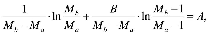 (E-3)
(E-3)
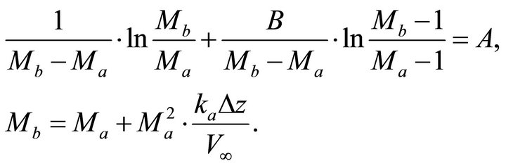
where A and B are known dimensionless parameters,
 (E-4)
(E-4)
The top asymptotic factor  is delivered by Equation (26), and the nonlinear Equation (E-4) should be solved for the unknown bottom asymptotic factor
 . To get the initial guess, we assume a small increment of the asymptotic factor on the interval,
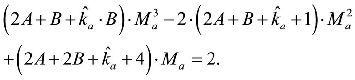
  , and expand Equation (E-3) into a power series. The cubic approximation reads
 (E-5)
(E-5)
where
 (E-6)
(E-6)
Equation (E-3) should be solved for .
.
Problem E2. RMS vs. depth with unknown velocity. Given data are the RMS velocities at the top and bottom interfaces,  and
and , the interval thickness
  and the top interface gradient
 . Find the top interface velocity
 . Solution. Use Equation (E-3) and the first equation of Equation Set (32),
 (E-7)
(E-7)
We solve Equation Set (E-7) for the unknown asymptotic factors  and
and . To obtain the initial guess for
 , assume that the increment of the asymptotic factor
 ![]() is small, and linearize Equation Set (E-7). This leads to
is small, and linearize Equation Set (E-7). This leads to
 (E-8)
(E-8)
Problem E3. RMS vs. time with unknown gradient. Given data are the RMS velocities at the top and bottom interfaces,  and
and , the interval traveltime
  and the top interface velocity
 . Find the top gradient
 . Solution. First we apply Equation (E-1) and calculate the hyperbolic parameter W. At this time, W is a known value. Next we apply Equation (48),
 (E-9)
(E-9)
where C is a known dimensionless parameter, the normalized local RMS velocity,
 (E-10)
and U is the non-normalized local RMS velocity on the interval. The top asymptotic factor  is delivered by Equation (26), and the bottom asymptotic factor
  is established from Equation (E-9). To solve this nonlinear equation, an initial guess is needed. Assume that the increment of the asymptotic factor
 ![]() on the interval is small, and expand Equation (E-9) into a power series. The cubic approximation reads
on the interval is small, and expand Equation (E-9) into a power series. The cubic approximation reads
 (E-11)
Problem E4. RMS vs. time with unknown velocity. Given data are the RMS velocities at the top and bottom interfaces,  and
and , the interval traveltime
  and the top interface gradient
 . Find the top interface velocity
 . Solution. We solve a set consisting of two equations: the first is Equation (E-9) combined with Equation (C-1), and the second is (C-1) itself,
 (E-12)
To get the initial guess, we linearize Equation Set (E- 12) for a small increment of the asymptotic factor ![]() and obtain
and obtain
 (E-13)
Problem E5. Depth vs. time with unknown gradient. Given data are the interval thickness , the traveltime
  and the top interface velocity
 . Find the top gradient
 . Solution. Use Equation (26) to find the top asymptotic factor
 . Next we apply Equation (37) to establish the bottom asymptotic factor
 (E-14)
where D is a known dimensionless parameter—the normalized interval velocity,
 (E15)
(E15)
To get the initial guess for Equation (E-14), we expand it into a power series for a small increment of the asymptotic factor![]() ,
,
 (E-16)
Equation (E-14) should be solved for the bottom asymptotic factor .
.
Problem E6. Depth vs. time with unknown velocity. Given data are the interval depth , the interval traveltime
  and the top interface gradient
 . Find the top interface velocity
 . Solution. Apply Equation (E-14) and the first equation of Equation Set (32),
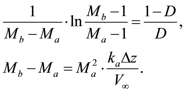 (E-17)
Next we solve Equation Set (E-17) for the unknown asymptotic factors  and
and . To obtain the initial guess, we linearize Equation Set (E-17) for a small increment of the asymptotic factor
![]() , and consider the first equation of the set,
, and consider the first equation of the set,
 (E-18)
Hence we obtain the initial guess for the top asymptotic factor ,
,
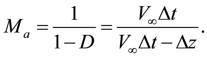 (E-19)
Problem E7. RMS vs. depth and time with unknown velocity and gradient. Given data are the RMS velocities at the top and bottom interfaces,  and
and , the interval traveltime
  and the interval thickness
 . Find the top interface velocity
  and gradient
 . Solution. The resolving set follows from Equations (E-9) and (E-14),
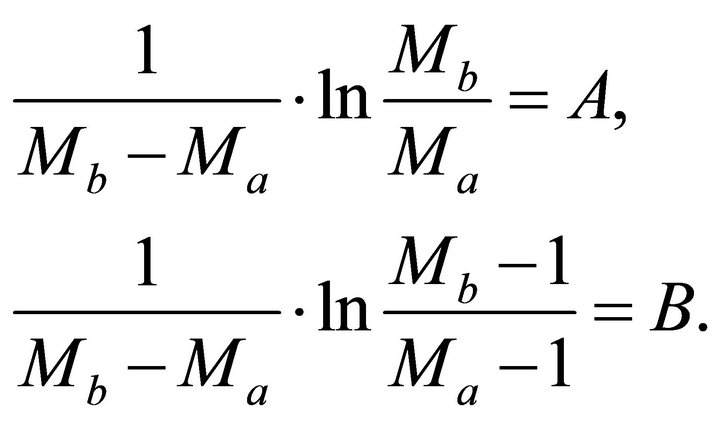 (E-20)
where A and B are known dimensionless parameters,
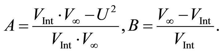 (E-21)
To obtain the initial guess, we assume that the top and bottom values of the asymptotic factor,  and
and , are close, and solve the two equations of Equation Set (E-20) apart. Each equation yields a root; the smaller root is the top asymptotic factor
 , and the larger root is the bottom asymptotic factor
 . The initial guess becomes
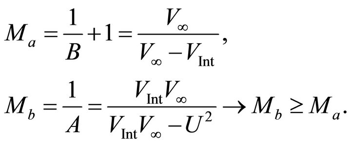 (E-22)
Appendix F. Three-Point Inversion
In this appendix we consider three problems where the RMS velocity is given at the interfaces and at an intermediate (inner) point of the interval vs. depth or time, or depth is given vs. time at the interfaces and at an intermediate point, and both parameters of the velocity profile,  and
and , are unknown.
Problem F1. RMS vs. depth with the unknown top interface velocity  and top gradient
 . Given data are the RMS velocities at the top and bottom interfaces,
  and
and , and the RMS velocity at the inner point of the interval,
  , the full interval thickness
  (between the top and bottom interfaces) and the partial thickness
  (between the top interface and the intermediate level). Find the top velocity
  and the gradient
 . Solution. The resolving equation set follows from Equation (E-3),
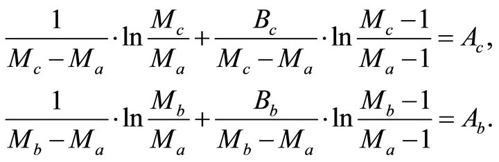 (F-1)
(F-1)
Coefficients  and
and  are known values; they follow from Equation (E-4),
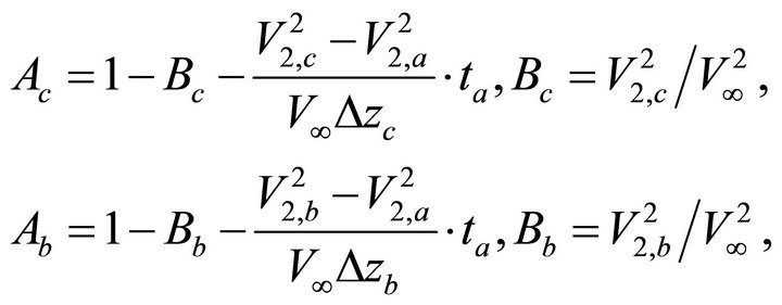 (F-2)
(F-2)
where the asymptotic factors  and
and  are to be found,
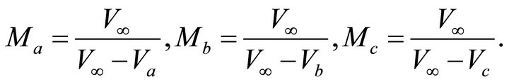 (F-3)
(F-3)
It follows from Equation (32),
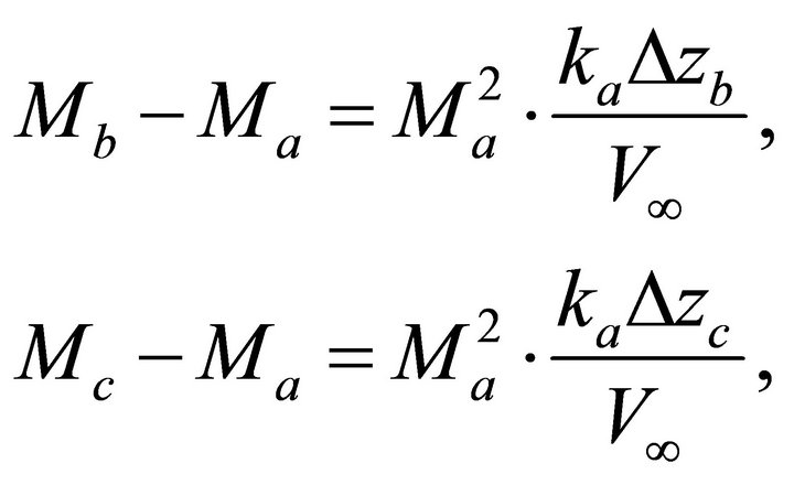 (F-4)
(F-4)
Divide the second equation of Equation Set (F-4) over its first equation,
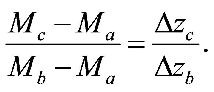 (F-5)
(F-5)
Thus, we solve Equation Set (F-1) together with Equation (F-5), to obtain the three unknown asymptotic factors. To obtain the initial guess, we assume that the layer is thin, i.e. that the differences in the asymptotic factors 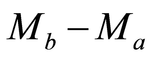 and
and 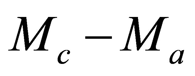 are small. This assumption allows linearization of Equation Set (F-1), which, in turn, results in
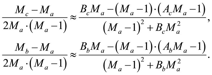 (F-6)
(F-6)
Introduction of solution (F-6) into Equation (F-5) leads to a fourth order polynomial equation for the top interface asymptotic factor ,
,
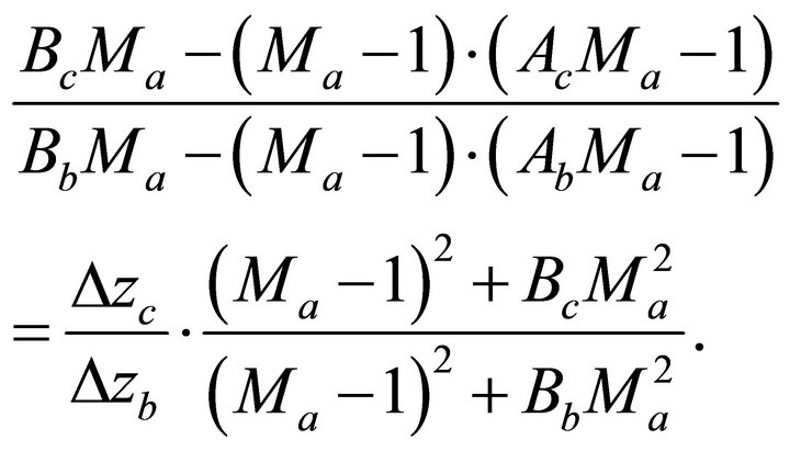 (F-7)
(F-7)
We solve Equation (F-7), choose a proper root, and this yields the initial guess for . Then we use Equation (F-6) to obtain the initial guess for
  and
and . Next we solve Equation Set (F-1), (F-5) numerically.
Problem F2. RMS vs. time with the unknown top interface velocity  and top gradient
 . Given data are the RMS velocities at the top and bottom interfaces,
  and
and , and at the inner point of the interval,
  , the full interval traveltime
  (between the top and bottom interfaces) and the partial traveltime
  (between the top interface and the intermediate level). Find the top velocity
  and the gradient
 . Solution. The resolving equation set follows from Equation (E-8),
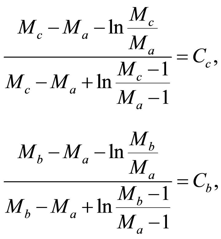 (F-8)
(F-8)
where  and
and  are the normalized local RMS velocities, for the partial interval and the full interval, respectively. These are the known dimensionless values,
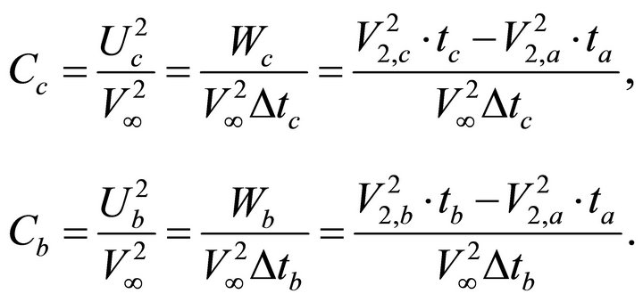 (F-9)
(F-9)
We make use of Equation (D-14),
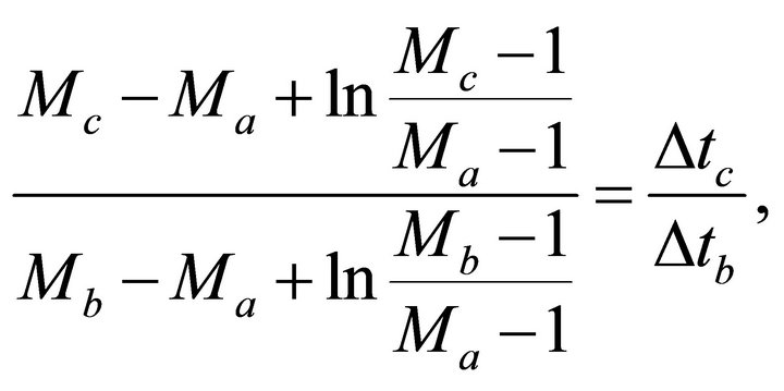 (F-10)
and solve Equation Set (F-8) numerically along with Equation (F-10). To obtain the initial guess, we assume that the layer is thin, and thus, we linearize Equation Set (F-8) for the small variations of the asymptotic factor,  and
and ,
,
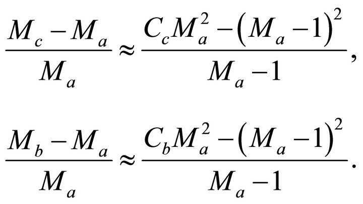 (F-11)
Note that for the small increments of the asymptotic factor
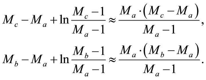 (F-12)
Linearization of Equation (F-10) leads to
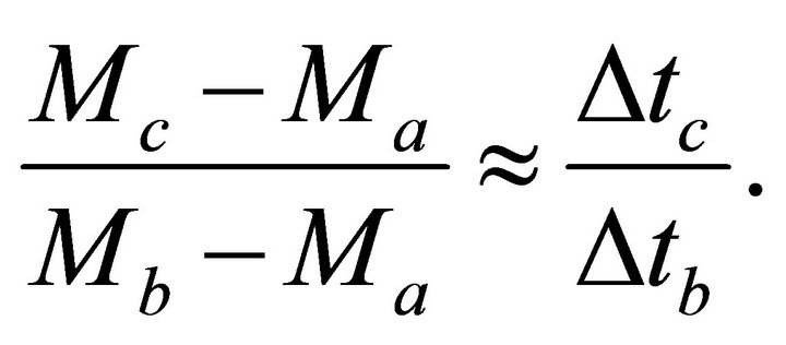 (F-13)
Equation (F-13) is similar to (F-5); however, (F-5) is exact and valid for any layer thickness, while (F-13) is an approximation for a thin layer only. Introduction of (F-13) into (F-11) results in a quadratic equation,
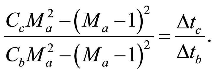 (F-14)
The equation has two positive roots, but only one of them exceeds 1. The solution is
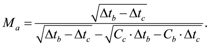 (F-15)
Next we apply Equation (F-11) to obtain the initial guess for  and
and . Then we solve Equation Set (F-8), (F-10) numerically and deliver the three asymptotic factors.
Problem F3. Depth vs. time with the unknown top interface velocity  and top gradient
 . Given data are the traveltime and layer thickness for the full and the partial intervals, respectively:
  and
and . Find the top velocity
  and the gradient
 . Solution. The resolving equation set follows from Equation (E-14),
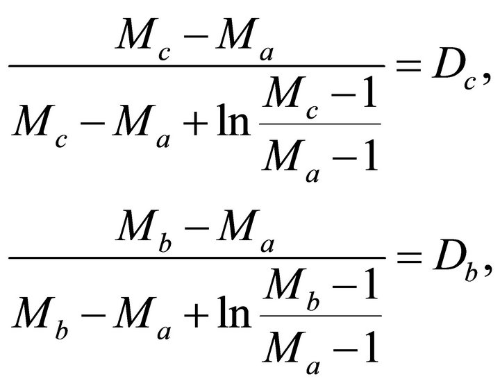 (F-16)
where  and
and  are the normalized interval velocities for the full and the partial intervals,
 (F-17)
Equation Set (F-16) should be solved numerically along with Equation (F-5). To obtain the initial guess, we linearize Equation Set (F-16) for the small increments of the asymptotic factors,
 (F-18)
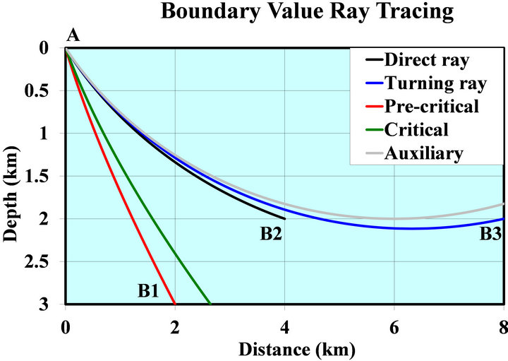
Figure 9. Boundary value ray tracing with the Hyperbolic velocity model: AB1—pre-critical ray, AB2—post-critical ray without the turning point, AB3—post-critical turning ray, green line-critical ray, grey line-auxiliary post-critical ray with the turning point at the given depth.
Introduction of Equation Set (F-18) into Equation (F-5) results in
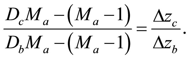 (F-19)
Equation (F-19) yields the initial guess for the top asymptotic factor ,
,
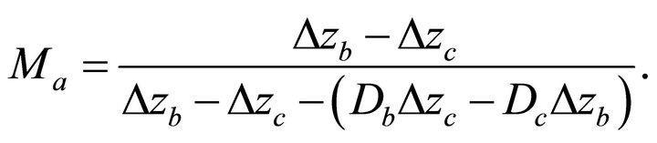 (F-20)
Equation (F-18) yields the initial guess for the bottom and the inner asymptotic factors,  and
and . Then we solve Equation Set (F-16) numerically, along with Equation (F-5).
Appendix G. Numerical Examples of BVRT
In this appendix, we present three examples of the boundary value ray tracing, Figure 9. The parameters of the velocity profile are the same as above. For each case, the source point  is located at the origin of the frame.
The destination point is different for each case: B1 (x = 2 km, z = 3 km), B2 (x = 4 km, z = 2 km), and B3 (x = 8 km, z = 2 km). As we will show, the first case corresponds to the pre-critical ray path, the second corresponds to the post-critical path that does not include the turning point, and the last case leads to the post-critical path with the turning point. First we calculate the critical lateral propagation with Equation (101): ΔxC = 1.587 km for the destination point depth zb = 2 km, and ΔxC = 2.646 km for zb = 3 km. Next we compare the horizontal offset  to the critical lateral propagation and apply the criterion in Equation (102):
  for the destination point B1 and
  for the destination points B2 and B3. We conclude that ray
  is pre-critical, while rays AB2 and AB3 are post-critical.
We solve Equation (105) for pre-critical ray  and establish its eccentricity:
 . The ray angles at the departure and the destination points are:
 and
and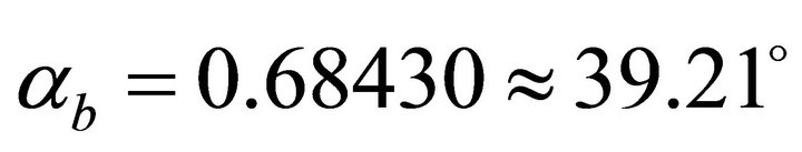 .
.
Next we figure out whether the post-critical rays ![]() and
and  include the turning point or not. If the postcritical ray includes a turning point, then the ray angle at the destination is obtuse, and this should be taken into account in Equation (104). For this we establish an auxiliary post-critical ray, whose maximum penetration depth is equal to the destination depth of points B1 and
 . We solve Equation (68) for the eccentricity,
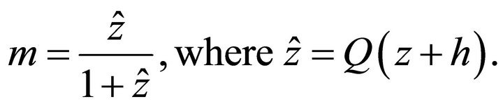 (G-1)
(G-1)
Compare Equation (G-1) with Equation (22). It is interesting to note that the eccentricity of a post-critical ray with the turning point at the given depth is equal to the normalized velocity at this depth. We obtain the eccentricity of the auxiliary ray , and the take-off angle
 . Calculate the half-chord of this ray with Equation (98),
 . Thus, we see that for the destination point
 , the offset is less than the half-chord of the auxiliary ray,
  , while for the destination point B3,
 . Hence we conclude that ray
 ![]() does not include the turning point, while ray
does not include the turning point, while ray  includes the turning point. We solve Equation (105) for ray
 ![]() and obtain the eccentricity,
and obtain the eccentricity,  , and the ray angles at the endpoints,
  For ray AB3 the results are:
 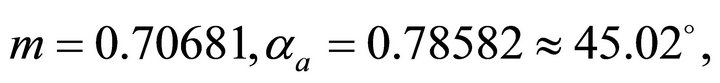 and
and 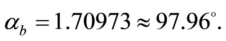 Note that the last angle is obtuse. The three traced rays, along with the auxiliary ray (grey line) and the critical ray (green line) are plotted in Figure 9.