International Journal of Geosciences
Vol.4 No.1(2013), Article ID:27012,11 pages DOI:10.4236/ijg.2013.41007
Calculation of Constitutive Parameters from Electric and Magnetic Field Measurements in an Anisotropic Medium with a Triaxial Instrument
Department of Geophysical Engineering, Kocaeli University, Kocaeli, Turkey
Email: ertanpeksen@kocaeli.edu.tr
Received August 8, 2012; revised September 24, 2012; accepted October 23, 2012
Keywords: Electrical Anisotropy; Triaxial Measurement; Electric and Magnetic Dipoles; Induction Well Logging
ABSTRACT
A hypothetical electric and magnetic induction tensor is considered in an anisotropic medium. The sources are magnetic dipoles. In such a medium, constitute parameters can be calculated by combining electric and magnetic field measurements. Constitutive parameters are not a scalar in this case. They are tensors, so parameters have at least both horizontal and vertical components in a uniaxial medium. These calculated parameters from the field measurement are horizontal and vertical conductivity, permittivity, and magnetic permeability. Operating frequency range is also quite large. It is up to 4 GHz. A hypothetical instrument should measure gradient fields both electric and magnetic types as well.
1. Introduction
Conductivity, permittivity, and permeability of a medium are known constitutive parameters [1]. These parameters are used to interpret the subsurface with different geophysical methods and well-logging types. Relative magnitudes of these parameters are quite distinct as very well-known properties of rocks [2-5]. Since these parameters seldom vary for most rocks and minerals, most scientists generally assume dielectric permittivity and magnetic permeability of the medium as free space for convenience. In an isotropic medium, constitutive parameters are the same in all directions; thus, they are scalars in that case. However, in an anisotropic medium these parameters depend on their directions, so they must at least be a vector. In the present study, an anisotropic medium is considered; thus, the determination of this kind medium requires five parameters in a vertical well. These are horizontal and vertical conductivities, permittivities, and magnetic permeability. This kind of anisotropy is known as a uniaxial anisotropy. In a Cartesian coordinate system, constitute parameters are the same in the x and y directions, but they are different in the z direction. If conductivity values are different in the x, y and z directions, this sort of medium is called as a biaxial medium.
In induction well logging, the electric anisotropy affects field measurements. Klein et al. [6] realized this effect and they stated that the possible reason for high reading could be the electrical anisotropy. Obviously, the effects of electrical anisotropy make interpretation erroneous. To deal with this effect and eliminate from the data, the electric anisotropy is considered.
In a wellbore, the field is also affected from a relative deviation angle. These effects can be included/extracted to/from the fields by rotating the Euler’s rotation matrix. Zhdanov et al. [7] studied the tensor well logging and they generalized Doll’s idea for an anisotropic medium. They showed that from the field components one can calculate not only conductivity values (horizontal and vertical) but also relative deviation and bearing angles. They used imaginary components of magnetic fields. Zhang et al. [8] showed that using field measurements one can determine relative angles such as relative dip and relative bearing as well. In general, there are three independent coordinate systems: a well, earth, and instrument coordinate systems. In this study, I consider a whole space (a uniaxial medium) and instrument axis are coincided with each other’s for the simplicity.
Many scientist [9-13] studied uniaxial media due to its simplicity. There have been a few authors studied a biaxial anisotropic medium, which can be characterized by its conductivity in each different directions in a Cartesian coordinate system [14-16].
A very few authors have studied electric field, and electric and magnetic field measurement together. Gribenko and Zhdanov [17] considered combination of electric and magnetic fields. They stated that the combination of the electric and magnetic field measurement gives better results with respect to conductivity distribution of a well. Here, the idea of combination of electric and magnetic field can be extended to an induction logging problem in an anisotropic medium.
In this study, I combine electric and magnetic fields in an anisotropic whole space. This is a hypothetical instrument. I demonstrate that constitutive parameters can be calculated by combining electric and magnetic field measurement in an anisotropic medium. Parameters are vertical and horizontal conductivities, dielectric permittivities, and magnetic permeability. These parameters characterize the field behaviors in a corresponding medium. In general, our aim is to measure field components and estimate those parameters, which characterize the field behaviors. In the present study, neither relative dip nor bearing is considered in the medium. In general, this hypothetical instrument should measure full electric and magnetic field components and their gradient in a well. Zhdanov [18] gave a definition of a gradient type measurement in an anisotropic medium for magnetic field. The same idea can also be extended to electric field measurement as well.
2. Maxwell’s Equations in an Anisotropic Medium
Moran and Gianzero [11] studied induction well logging in a uniaxial anisotropic medium. Maxwell’s equations are given in such a medium as:
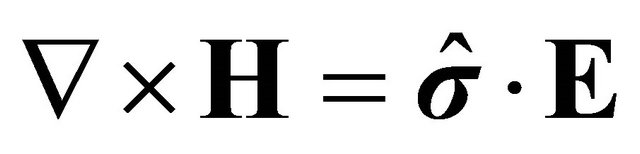 , (1)
, (1)
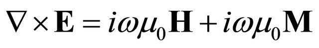 , (2)
, (2)
where E is the electric field (V/m), H is the magnetic field (A/m). M is a magnetic dipole moment (Am2). The conductivity tensor in a transversely isotropic (TI) medium is:
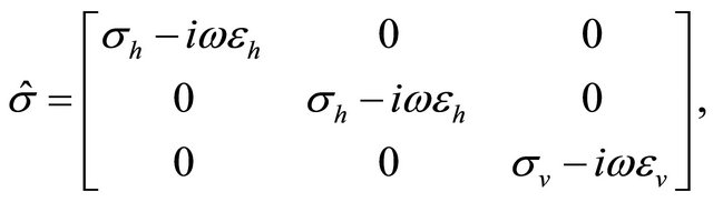 (3)
(3)
where  is the horizontal component and
  is the vertical component of conductivity tensor.
  and
and  are the horizontal and vertical permittivity of the medium, respectively. The free space dielectric permittivity is
  F/m. The free space magnetic permeability is
  H/m. The transverse isotropic medium is excited through an electromagnetic field generated by magnetic dipoles with unit moments. The time dependence is
  f is the frequency of a source in Hertz.
Moran and Gianzero [11] solved Equations (1) and (2) by using the Hertz potential. In this paper, I assume that the dielectric permittivity and magnetic permeability of the medium are not free space. In this situation, electric and magnetic field components can be written:
 , (4)
, (4)
 , (5)
, (5)
where  is a Hertz vector and
  is a scalar potential. The medium dielectric permittivity and magnetic permeability are
 ,
,  and
and , respectively.
  and
and  stand for the relative dielectric permittivity,
  represents a relative magnetic permeability. Super and subscripts depict a magnetic moment and receiver direction along the corresponding axis; thus, n and m can be x, y, and z, in Equations (4) and (5).
In this paper, I use as the following notation: Bold face symbols or characters with a hat stand for tensors, while bold face symbols or characters without a hat illustrate vectors. Any characters with italic are a scalar. Therefore, calculations involve some dyad algebra such as dyadicvector dot product in Equations (4) and (5). Next two sections investigate electric and magnetic field components.
3. Electric Induction Tensor
Electric induction tensor has 9 components in a general case. Three orthogonal receivers and transmitters are elongated with their corresponding axis in a Cartesian coordinate system. The sources are magnetic dipoles and receivers are electromagnetic sensor or coils. To derive the electric field components is a straightforward calculation that will not be repeated here. Reader can find all electric components from [19-21].
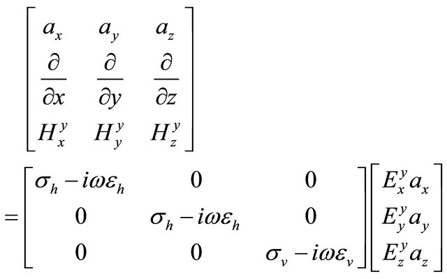
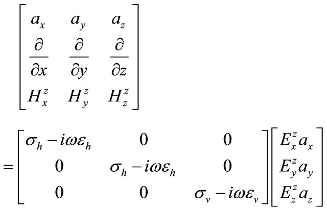
The electric induction tensor can be represented in a matrix form as:
 , (6)
, (6)
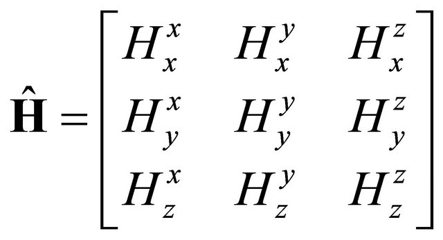
where superscripts are magnetic dipole orientations and subscripts are receiver orientations. Bear in mind that the sources are magnetic dipoles. Figure 1 displays a hypothetical electric and magnetic induction tensor. Figure 2 shows the behavior of electric field components in a x-y plane. For field simulation, the horizontal and vertical conductivities are 0.1 and 0.025 S/m, respectively. The operating frequency is 20 kHz. The field computation is conducted with free space dielectric permeability and magnetic permeability. M is a magnetic dipole with a unit. One can realize that the symmetrical fields have the same amplitude, but different sings.
4. Magnetic Induction Tensor
In this section, a magnetic induction tensor is investigated. As the electric induction tensor, the magnetic in-
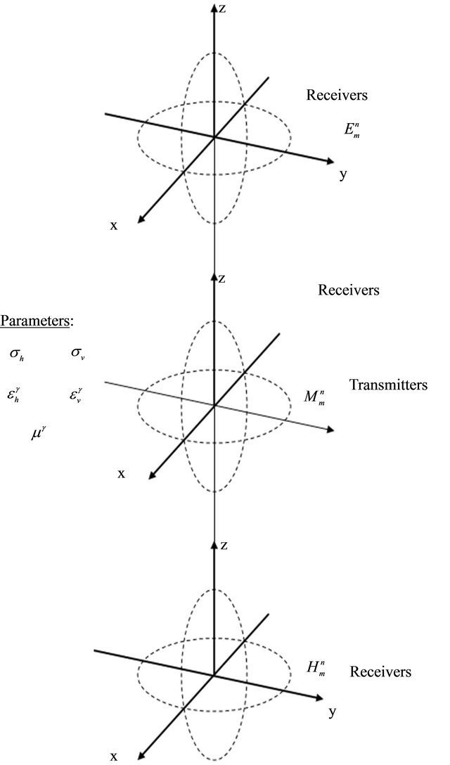
Figure 1. A sketch of a triaxial induction logging instrument is in a well. The physical medium properties are conductivity, dielectric permittivity, and magnetic permeability. The sources are magnetic dipoles. Receives are both magnetic and electric field sensors. Super and subscripts indicate the direction of transmitter and receiver, respectively (n and m can be x, y and z). Conductivity and dielectric permittivity are tensors, since they have principal values at least two values. The magnetic permeability is assumed a scalar.
duction tensor has also 9 components. It can be shown in a matrix form as:
 , (7)
, (7)
where the notation is the same as the electric induction tensor. Three transmitter and receiver coils are oriented along the x, y, and z-axes in a Cartesian coordinate system. Derivation of magnetic field components is a straightforward calculation that will not be repeated here. Magnetic field of analytic components can be found from [7,22].
The magnetic induction tensor is symmetric. Behavior of magnetic field components is displayed in Figure 3. The uniaxial model parameters are the same as the previous electric field calculation. Thanks to commercially available 3DEX and Rt Scanner induction well logging instruments reads a lot of data at different frequencies for various field components. That means considerable amount of data are available. From 3DEX and Rt Scanner data, conductivities, relative dip and bearing angles can be estimated [8].
In Figure 4, each components of magnetic induction tensor are displayed in volumetric 3-D at 20 kHz. In all panels, imaginary parts of the magnetic field are normalized by absolute value of the corresponding components. The medium conductivities are:  1/40 S/m and
  1/80 S/m. To able to see all panels, 0.1 value used for off diagonal components. As for diagonal components, I use 0.0045 value. Red and blue colors show sign. Blue used for negative, while red used for positive values. The behaviors of components are quite different from each other’s.
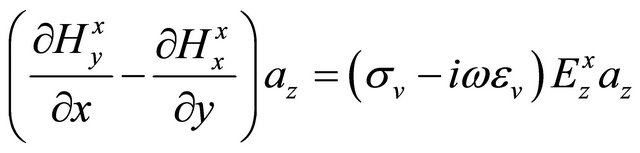
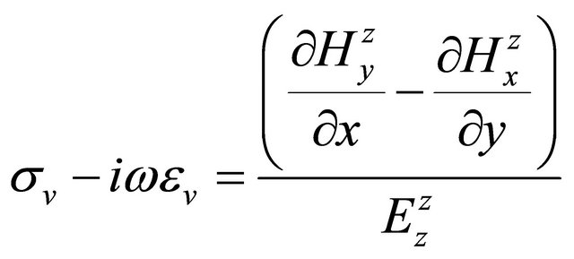
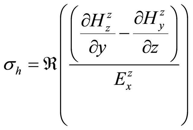
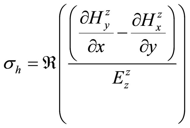
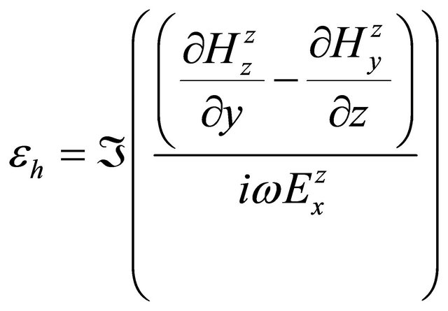
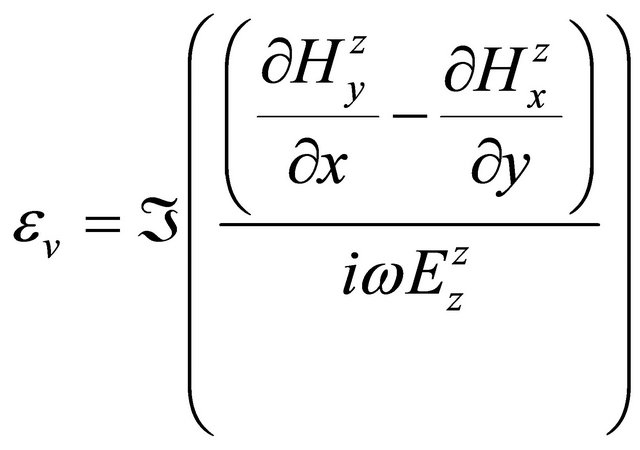
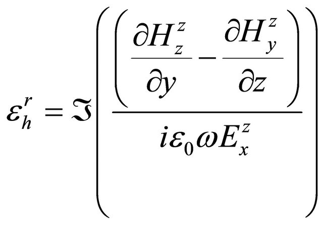
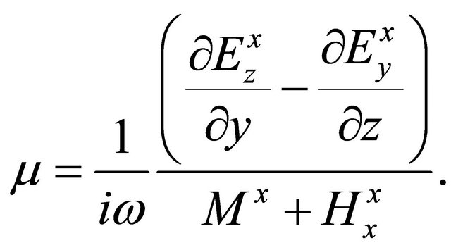
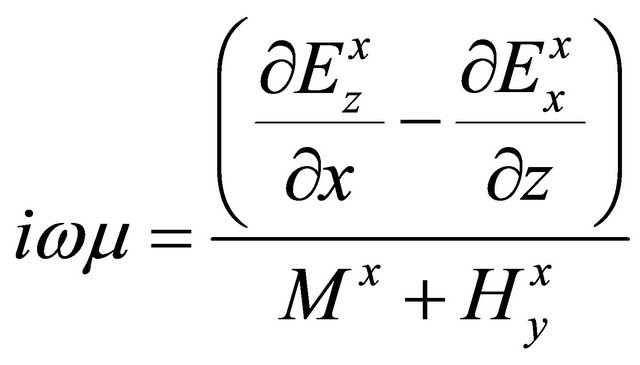
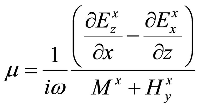
5. Estimation of Earth Parameters: Conductivity, Dielectric Permittivity, and Magnetic Permeability
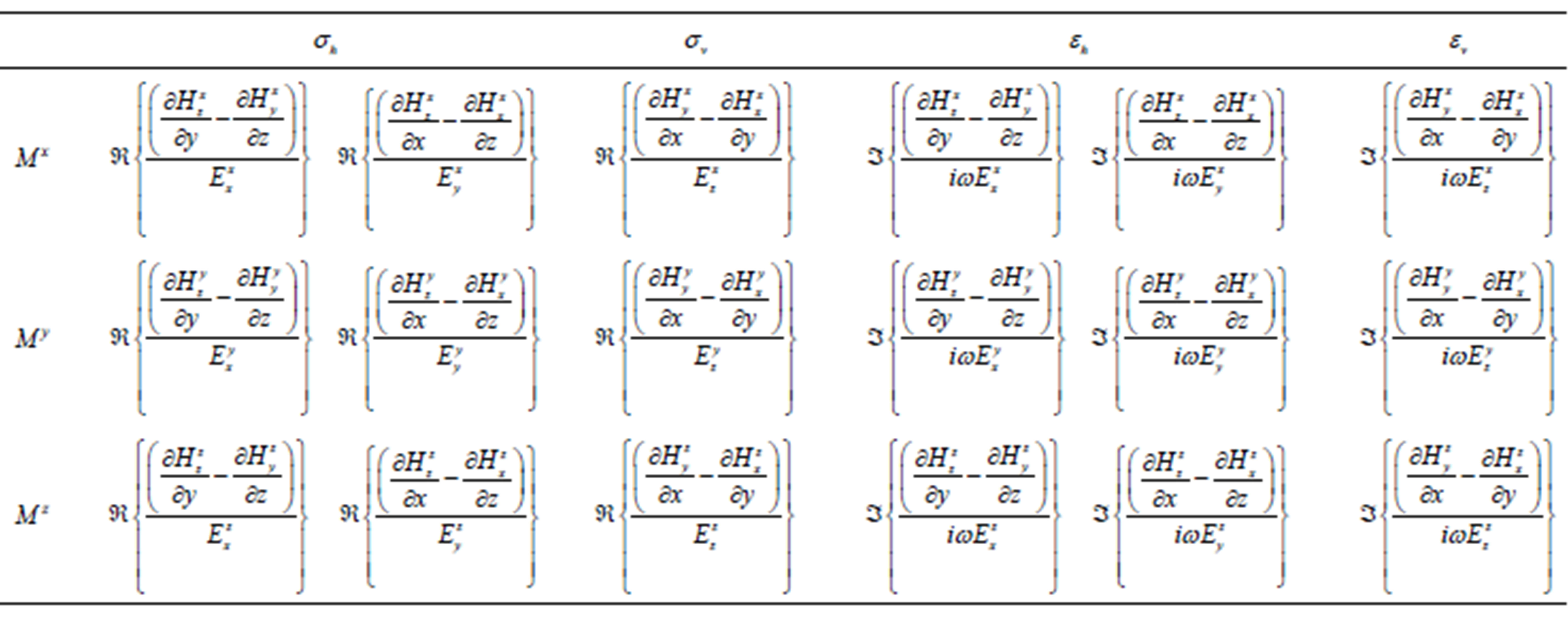
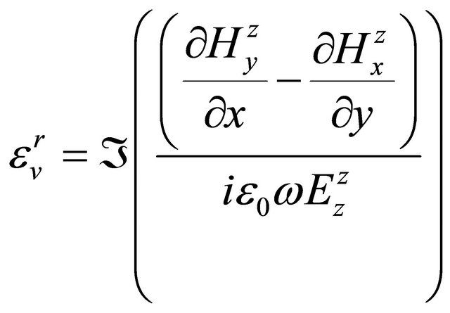
I consider a hypothetical multi-component induction well logging instrument. As mentioned previously, the instrument has magnetic dipoles as a source in the x, y and z directions. Receivers should measure magnetic and electric field components. It is a combination of electric and magnetic induction tensor components. It requires some tensor-gradient measurements. From this hypothetical electric and magnetic induction tensor-gradient measurement, one can estimate earth (or formation) parameters. There are many different formulas are given in Table 1. In the first column of the table is a magnetic moment direction, while the first row depicts earth parameters. A simple derivation is given in Appendix A. From Table 1, it is easy to see that there are many different formulas for estimating the earth parameters. One can calculate conductivities and dielectric permitivities in the horizontal and vertical directions. These formulas can be useful when one of these components is very noise, the other one can be used for calculating the corresponding earth parameters in a practical situation. They may be useful for checking parameters against each other using different field measurements. This method will obviously increase the quality of the formation evaluation. Table 1 has formulas for conductivities and dielectric permittivities. Appendix B derives formulas for magnetic permeability. These formulas are given in Table 2. In both tables,  and
and  stand for real and imaginary components of the corresponding field, respectively.
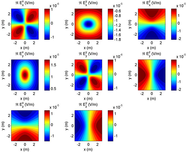
Figure 2. Real parts of the magnetic field components are calculated in an anisotropic medium with 20 kHz operating frequencies at z = 1 m. The horizontal and vertical conductivities are 1/40 and 1/80 S/m, respectively. It is a top view of a whole space.
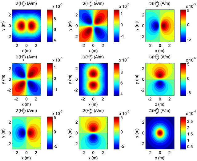
Figure 3. Imaginary parts of the magnetic field components are calculated in an anisotropic medium with 20 kHz operating frequencies at z = 1 m. The horizontal and vertical conductivities are 1/40 and 1/80 S/m, respectively. It is a top view of the medium.
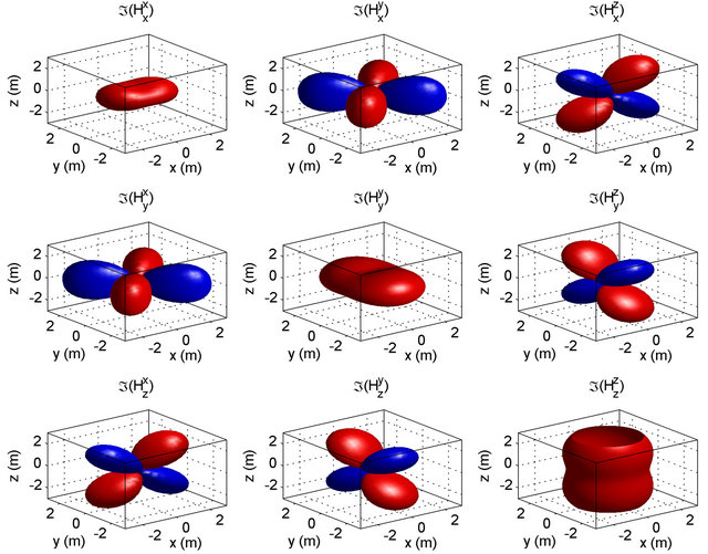
Figure 4. Volumetric 3-D representation of the magnetic tensor components at value 0.1 (off diagonal) and 0.0045 (diagonal). The medium is conducted with σh = 1/40 S/m and σh = 1/80 S/m. Blue colors display negative, while red ones depict positive values of imaginary part of the magnetic field.
Table 1. Magnetic moments are in the first column. The superscripts show the direction of the magnetic moments. The rest of the formulas are apparent conductivities and dielectric permittivities.  and
and  depict for real and imaginary components of the corresponding field.
Numerical Example
In a uniaxial medium, I consider as the following parameters for numerical calculation: 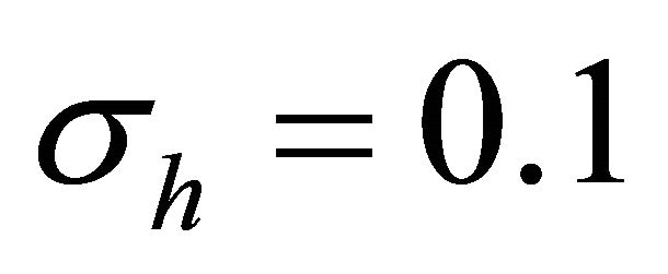 and
and 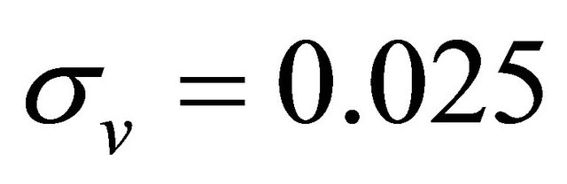 S/m;
S/m; 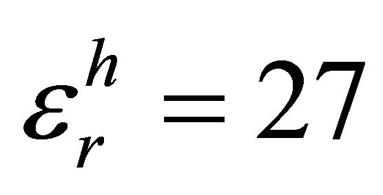 and
and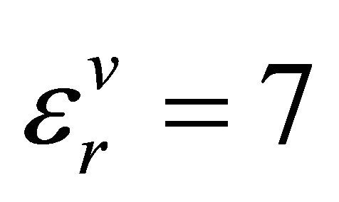 ;
; . The frequency range for calculation begins at 10 kHz and it expands up to 4 GHz. The distance between transmitter and receivers is 1.6 m as a typical induction T-R distance.
The model response in a whole space is calculated by a magnetic dipole oriented in the y direction. Electric and magnetic field components and their space derivatives are calculated by using analytic formulas. For constitute parameter calculation, a group of the formulas given in Table 1 are used, which are on the second rows. All parameters are related to a uniaxial medium estimated, correctly. Figure 5 displays the result. Note that these are
Table 2. Magnetic moments are in the first column. The superscripts show the direction of the magnetic moments. All formulas in the table can be used for calculating apparent magnetic permeability.
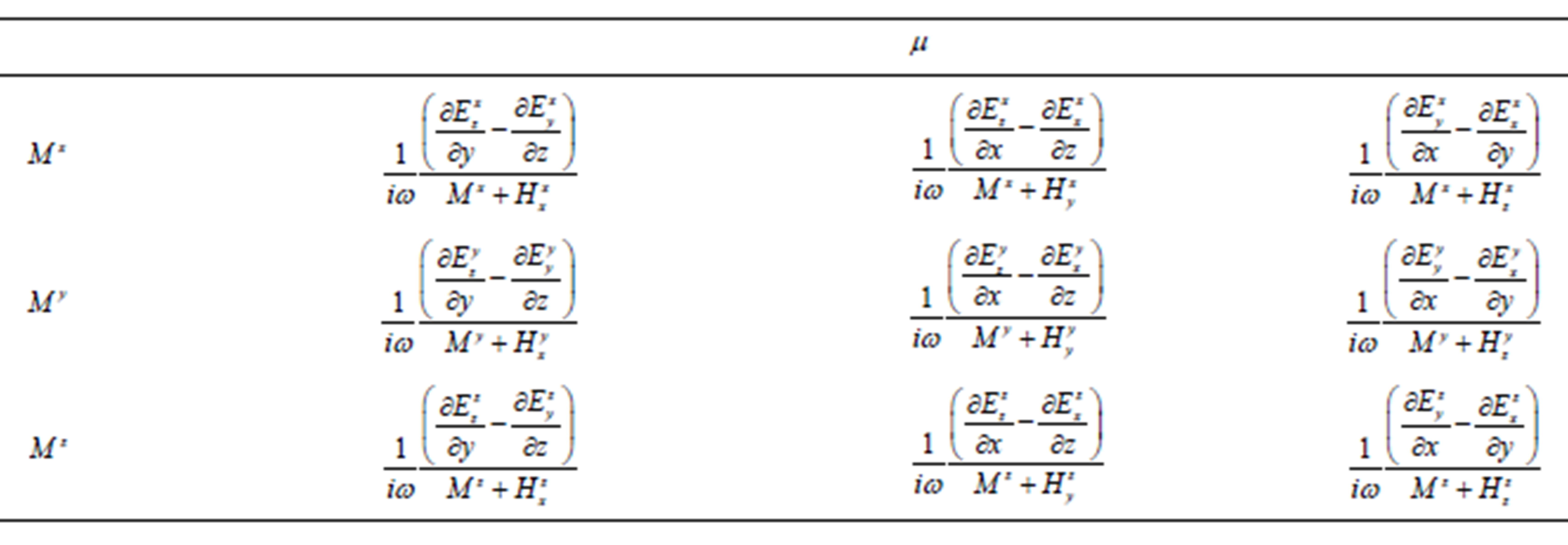
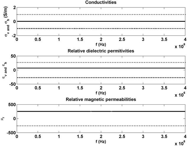
Figure 5. Constitutive parameters are horizontal and vertical conductivity, relative dielectric permittivity and magnetic permeability of the medium. The magnetic moment direction is in the y direction. On each panel, solid, dotted, and dashed lines show the result. The calculation done with the formulas are given on the second row in Table 1. Solid lines illustrate horizontal values of both conductivity and dielectric, while dotted and dashed lines display vertical values of those parameters. The frequency range is quite large between at 10 kHz and 4 GHz. The medium has conductivity values with σh = 0.1 and σv = 0.025 S/m; relative dielectric values with  and
and ; and relative magnetic permeability μr = 255. The distance transmitter and receivers is 1.6 m as a typical induction T-R distance.
only some simple formulas in Tables 1 and 2. I do not use any kind of optimization techniques. However, the formulas require some gradient type measurement not only for magnetic, but also electric field.
In Figure 5, dotted and dashed lines show horizontal parameters on the first and in the middle panels. There are two formulas in Table 1 in the middle panel. When one use the upper formula, the result is negative. This is illustrated with dashed lines. The lower formula gives positive values. This is showed with dotted lines. As for the horizontal parameters, they are depicted with a solid line in Figure 5. As seen from Table 1, the real parts of the formulas give conductivity values. Dielectric values can be calculated from the imaginary parts of the formulas.
6. Conclusion
I have considered a hypothetical induction instrument in a uniaxial medium. In such a medium, one can calculate constitutive parameters such as conductivity, dielectric permittivity, and magnetic permeability. Nowadays, 3DEX and Rt Scanner technology is quit mature, but considered a suggested hypothetical instrument may be useful for formation evaluation since conductivity, dielectric permittivity and magnetic permeability values are important with respect to petrophysical parameters, because they are related to water saturation, porosity, and permeability. The formulas developed the present study are exact, since they have derived from Maxwell’s equations. I have not used any kind of approximation in order to derive these parameters. Application of this method requires some gradient type field measurement, which might be the most difficult part of this application.
REFERENCES
- C. A. Balanis, “Advanced Engineering Electromagnetics,” John Wiley & Sons, Inc., Hoboken, 1989.
- R. S. Carmichael, “Practical Handbook of Physical Properties of Rocks and Minerals,” CRC, Boca Raton, 1989.
- F. S. Grant and G. F. West, “Interpretation Theory in Applied Geophysics,” McGraw-Hill Book Company, New York, 1965.
- M. N. Nabighian, Ed., “Electromagnetic Methods in Applied Geophysics V. I: Theory,” SAGE Publication, Thousand Oaks, 1987.
- M. S. Zhdanov and G. V. Keller, “The Geoelectrical Methods in Geophysical Exploration,” Elsevier, Amsterdam, 1994.
- J. D. Klein, P. R. Martin and D. F. Allen, “The Petrophysics of Electrically Anisotropic Reservoirs,” SPWLA 36th Annual Logging Symposium, Paris, 26-29 June 1995, Paper HH.
- M. S. Zhdanov, D. Kennedy and E. Peksen, “Foundations of Tensor Induction Well-Logging,” Petrophysics, Vol. 42, No. 6, 2001, pp. 588-610.
- Z. Zhang, L. Yu, B. Kriegshauser and L. Tabarovsky, “Determination of Relative Angles and Anisotropic Resistivity Using Multicomponent Induction Logging Data,” Geophysics, Vol. 69, No. 4, 2004, pp. 898-908. doi:10.1190/1.1778233
- B. I. Anderson, T. D. Barber and M. G. Lulling, “The Response of Induction Tools to Dipping Anisotropic Formations,” SPWLA 36th Annual Logging Symposium, Paris, 26-29 June 1995, Paper D.
- M. G. Lüling, R. Rosthal and F. Shray, “Processing and Modeling 2 MHz Tools in Dipping, Laminated Anisotropic Formations,” SPWLA 35th Annual Logging Symposium, Tulsa, 19-22 June 1994, Paper QQ.
- J. H. Moran and S. C. Gianzero, “Effects of Formation Anisotropy on Resistivity Logging Measurements,” Geophysics, Vol. 44, No. 7, 1979, pp. 1266-1286. doi:10.1190/1.1441006
- L. Zhong, C. L. Shen, R. Liu, M. Bittar and G. Hu, “Simulation of Tri-Axial Induction Logging Tools in Layered Anisotropic Dipping Formations,” 76th Annual International Meeting SEG, New Orleans, 2006, pp. 456- 460.
- L. L. Zhong, J. Li, L. C. Shen and R. C. Liu, “Computation of Triaxial Induction Logging Tools in Layered Anisotropic Dipping Formations,” IEEE Transactions on Geoscience and Remote Sensing, Vol. 46, No. 4, 2008, pp. 1148-1163. doi:10.1109/TGRS.2008.915749.
- S. Gianzero, D. Kennedy, L. Gao and L. San Martin, “The Response of a Triaxial Sonde in a Biaxial Anisotropic Medium,” Petrophysics, Vol. 43, No. 3, 2002, pp. 172- 184.
- A. G. Nekut, “Anisotropy Induction Logging,” Geophysics, Vol. 59, No. 3, 1994, pp. 345-350. doi:10.1190/1.1443596
- N. Yuan, X. C. Nie, R. Liu and C. W. Qiu, “Simulation of Full Responses of a Triaxial Induction Tool in a Homogeneous Biaxial Anisotropic Formation,” Geophysics, Vol. 75, No. 2, 2010, pp. E101-E114. doi:10.1190/1.3336959
- A. Gribenko and M. S. Zhdanov, “Rigorous 3D Inversion of Tensor Electrical and Magnetic Induction Well Logging Data Inhomogeneous Media,” 79th Annual International Meeting SEG, Houston, 2009, pp. 431-435.
- M. S. Zhdanov, “Method and Apparatus for Gradient Electromagnetic Induction Well Logging,” PCT WO 2005/ 083467 A1. 2005.
- X. Lu, D. L. Alumbaugh and C. J. Weiss, “The Electric Fields and Currents Produced by Induction Logging Instruments in Anisotropic Media,” Geophysics, Vol. 67, No. 2, 2002, pp. 478-483. doi:10.1190/1.1468607
- E. Peksen, “Methods for Interpretation of Tensor Induction Well Logging in Layered Anisotropic Formations,” Ph.D. Thesis, University of Utah, Salt Lake City, 2004.
- T. Wang, “The Electromagnetic Smoke Ring in a Transversely Isotropic Medium,” Geophysics, Vol. 67, No. 6, 2002, pp. 1779-1789.
- M. Rabinovich, L. Tabarovsky, B. Corley, L. van der Horst and M. Epov, “Processing Multi-Component Induction Data for Formation Dips and Anisotropy,” Petrophysics, Vol. 47, No. 6, 2006, pp. 506-526. doi:10.1190/1.1527078
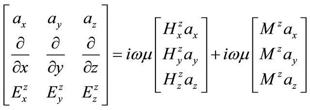
Appendix A
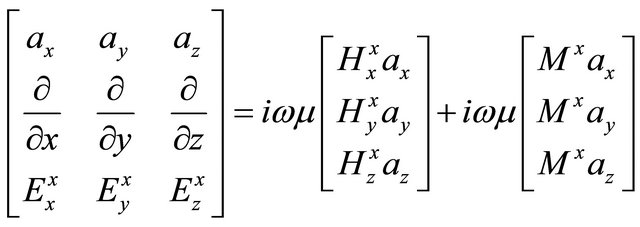
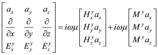
Equation (1) can explicitly be written
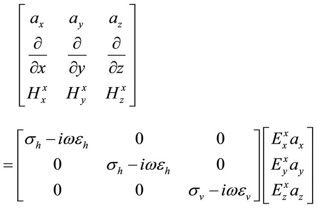 , (A.1)
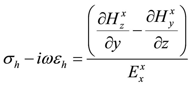
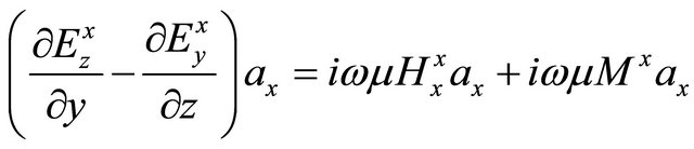
where ax, ay and az are the unit vectors in a Cartesian coordinate system. H and E are the components of corresponding fields either magnetic or electric. Superscripts stand for the magnetic moment direction, while subscripts stand for the field directions. The first, the electric and magnetic field components will be considered generated by an x-directed magnetic dipole. For this purpose, I rewrite Equation (A.1) and I have T
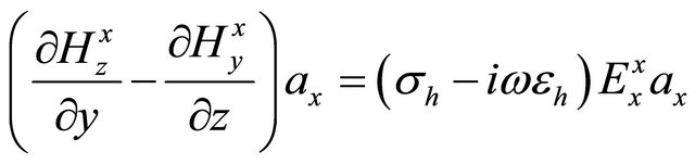 , (A.2)
 , (A.3)
and
 . (A.4)
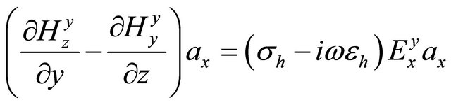
Equations (A.2), (A.3) and (A.4) allow us to estimate horizontal and vertical conductivities from electric and magnetic fields. Continuing derivation yields
 , (A.5)
 , (A.6)
and
 . (A.7)
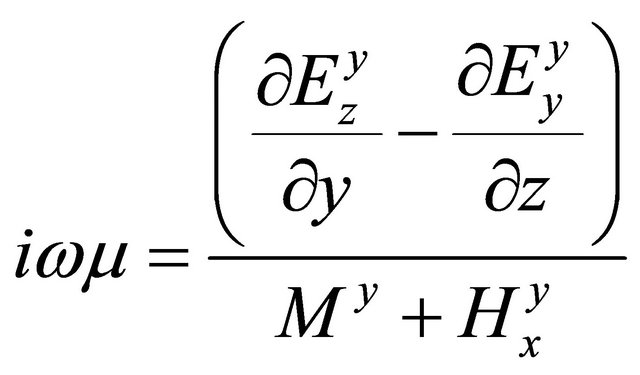
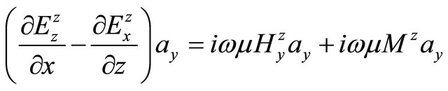
The real part of Equations (A.5), (A.6) and (A.7) gives conductivity and the imaginary part of the same equation yields to permittivity. Continuing setting up Table 1, electric-magnetic field components generated by a y-directed magnetic dipole gives three more formulas. Let us look at Equation (1) again,
 , (A.8)
and from Equation (A.8) I can write as the following equations,
 , (A.9)
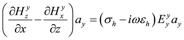 , (A.10)
and
 . (A.11)
Then parameters can be estimated as the following expressions
 , (A.12)
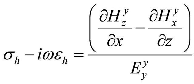 , (A.13)
and
 . (A.14)
Conductivities can be calculated from the real part of Equations (A.12), (A.13) and (A.14) and the imaginary part of the same equation may be used for estimating dielectric constant.
Further derivation using a z-directed magnetic dipole gives three more formulas. Let continue the derivation from Equation (1),
 . (A.15)
Proceeding with some very simple algebra allows us to have other parameters. From Equation (A.15) it is very easy to have
 , (A.16)
 , (A.17)
and
 . (A.18)
Again, having conductivities and dielectric permittivites are easy. From the last three equations I can derive as the following expressions:
 , (A.19)
 , (A.20)
and
 . (A.21)
From Equations (A.5), (A.6), (A.7), (A.8), (A.9), (A.10), (A.12), (A.13), and (A.14) apparent conductivity and permittivity can be calculated. For this purpose, the real part of the Equations (A.19) and (A.20) are used. Horizontal and vertical conductivities may be estimated with
 , (A.22)
 . (A.23)
Similar to previous two formulas, apparent dielectric permittivities can be
 , (A.24)
and
 . (A.25)
Further, consider relative permittivity as  and
and  and rewrite the last two equations, I have
 (A.26)
and
 . (A.27)
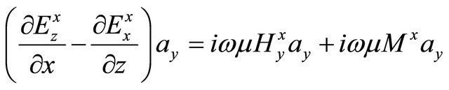
Appendix B
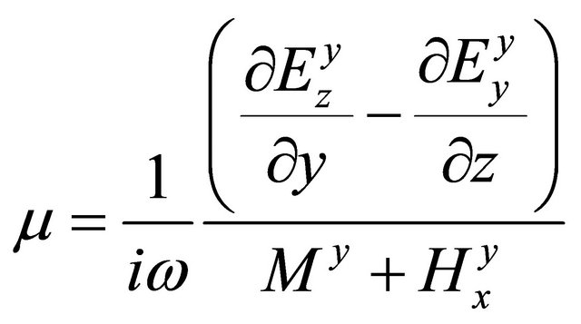
The formulas for the magnetic permeability estimation can be derived by using Equation (2). Rewrite Equation (2) explicitly with x directed a magnetic dipole. Bear in mind that the magnetic permeability is scalar. I can write it as
 . (A.28)
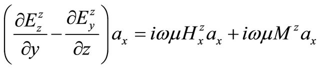
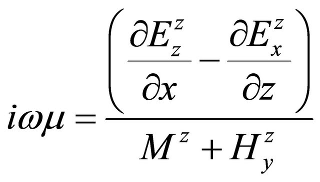
The first component of Equation (A.28) with x-directed magnetic dipole with M a unit moment, from the previous step I can proceed with
 , (A.29)
and keep on derivation, which yields
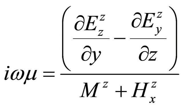
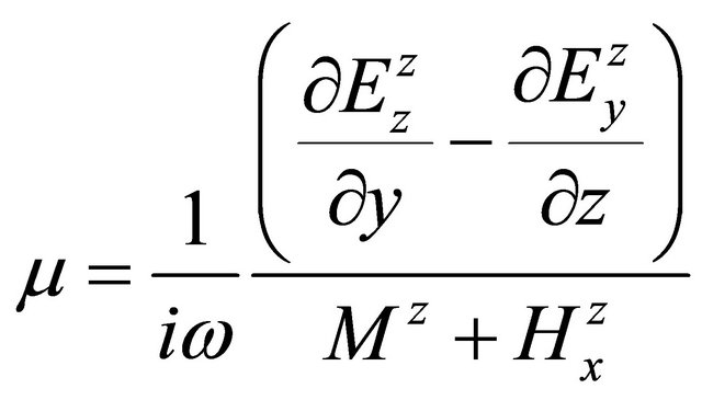
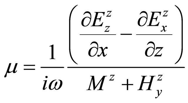
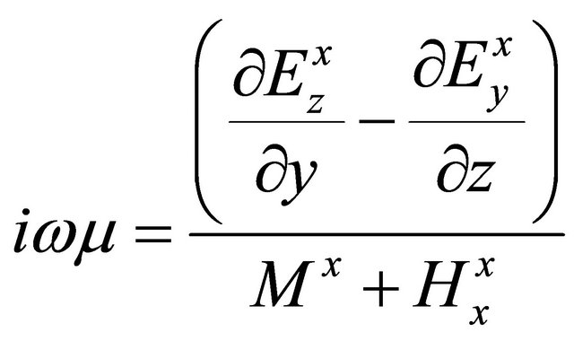 . (A.30)
From Equation (A.30), it is easy to have magnetic permeability:
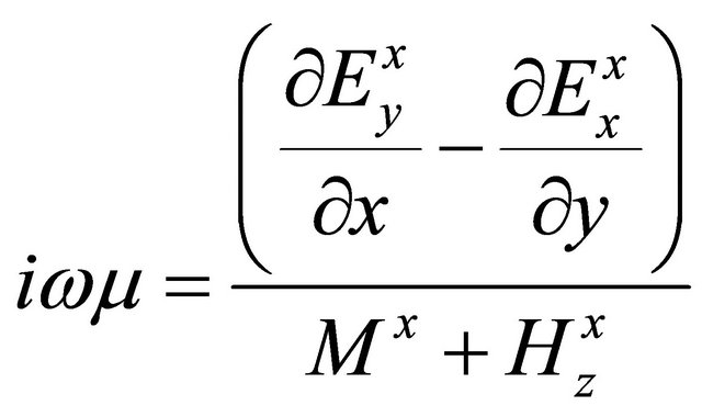
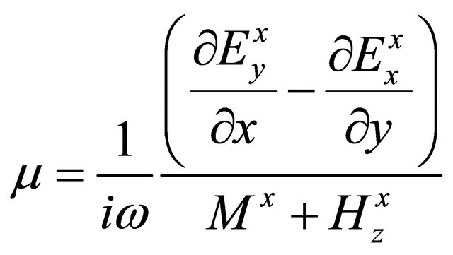
 (A.31)
It can be derived some formulas for the magnetic permeability by using the same procedure as on the previous component derivation.
 (A.32)
 , (A.33)
 . (A.34)
From the last component of the corresponding vector, one can get
 . (A.35)
 , (A.36)
and
 . (A.37)
Then, carry on the derivation
 , (A.38)
 , (A.39)
 , (A.40)
yields one more formula for the magnetic permeability of the medium, which is
 . (A.41)
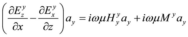
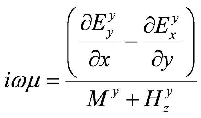
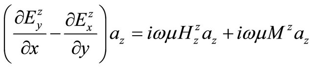
Considering the y component of the vector, then keep on
 (A.42)
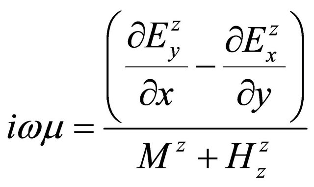
which yields
 , (A.43)
then it is easy to have
 . (A.44)
When I apply similar procedure, the rest of the magnetic formulas may be derived:
 , (A.45)
 , (A.46)
 . (A.47)
 , (A.48)
 , (A.49)
 , (A.50)
 . (A.51)
 , (A.52)
 , (A.53)
 . (A.54)
 , (A.55)
 , (A.56)
and
 . (A.57)