International Journal of Geosciences
Vol. 3 No. 3 (2012) , Article ID: 21217 , 8 pages DOI:10.4236/ijg.2012.33053
A New Shrinkage Curve Model, Applied to Moroccan Clayey Soil
1Ecole Mohammadia d’Ingénieurs, UM5-Agdal, Rabat, Morocco
2Laboratoire Public d’Essais et d’Etudes, Casablanca, Morocco
Email: s_bensallam@yahoo.fr
Received February 29, 2012; revised March 30, 3012; accepted May 2, 2012
Keywords: Clayey Soil; Expansive Soil; Shrinkage Curve; Analytical Model
ABSTRACT
On the basis of the existing relation between the soil’s water content and its structural evolution, we elaborate a new analytical model allowing the analysis of the soil’s shrinkage curve according to the limits of its hydro-structural boundaries. This model was conducted on undisturbed clayey soil at Moulel-Bergui, Morocco.
1. Introduction
The action of the argillaceous phase on the hydro-mechanical soil properties is globally recognized. And the abundance of this expansive soil at the global scale generated too many efforts in order to better understand their behavior. In the field, these kinds of soils are basically non-homogeneous and their hydro-mechanical properties are argillaceous phase depending, giving them the capacity to vary the soil’s volume according to its water content.
Most studies of the clay soil’s volume change are focused on their swelling character, but the shrinkage character still lacks study. The aim of this paper is to give an analytical approach to describe the shrinkage process, by using some modified laboratory tests on the basis of the existing relation between the evolution of the shrinkage process and the structural variations which accompany it.
In addition to the conventional laboratory mechanical tests, the shrinkage curve analysis seems to be the best way to follow up the evolution of the hydro-structural soil’s properties during the drying process. Indeed, the shrinkage curve analysis is one of the rare methods which makes it possible to describe the quantitative evolution of the clay soil hydro-structural properties. Because there is no conventional model unanimously used to describe the shrinkage curve, this paper proposes an analytical model to describe the clay soil’s behavior during the desaturation phase.
2. Theory
2.1. Shrinkage Curve Description
Usually, the superficial clay soils are non-rigid and nonhomogeneous and the transfer of water through this system is done via the argillaceous matrix porosity and its cracks network caused by the shrinkage. The knowledge of the shrinkage rate of these soils is required to understand their hydro-mechanicals behavior.
Basically, the clay’s volume is moisture depending. During the drying process, the clay volume decreases when the medium moisture decreases with a rearrangement of the particles and the aggregates. These modifications of the soil structure influence the displacement of the interstitial solutions in the soil matrix, making its transport more complex compared with the rigid soils. To determine how the soil’s volume decreases during drying, the behavior of the soil shrinkage can be characterized either by its void ratio according to its moisture state [1-4] or by its specific volume according to its water content [5,6]. For our study we chose to use the variation of the void ratio (e) according to the water content (W).
The shrinkage curve is characterized by four clear-cut phases (Figure 1). From the wet side of the curve to the dry side, these phases are: the Structural shrinkage, the Normal shrinkage, the Residual shrinkage and the Zero shrinkage. In the zone of structural and residual shrinkage, the soil’s volume reduction is smaller than the quantity of water extracted from the medium. In the structural phase, the water extracted is exclusively the free water localized out of the action sphere of the particles. In the zone of normal shrinkage, the volume reduction is almost equal to the quantity of extracted water, and during this stage the air volume in the medium remains constant in the soil’s matrix [4,6]. In the zone of zero shrinkage the volume does not change any more, except if there is a disintegration of particles creating a new micro-porosity
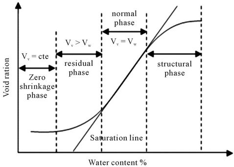
Figure 1. Representation of the shrinkage curve phases.
and leading to a new rearrangement of particles. However, all the clay soils do not always show those four shrinkage zones. In some cases the shrinkage curve does not present the zone of structural shrinkage (Kim et al. 1999); in other cases, it is the phase of zero shrinkage which is absent (McGarry and Malafant, 1987).
Each shrinkage phase is delimited by a boundary limit and corresponds to a particular configuration of the soil with a particular morphology and properties at the microscopic and the macroscopic scale.
As has been noted before, the use of the shrinkage curve allows to evaluate the volume changes according to the water content, and to determine the active specific volume in the soil mass by the means of the active argillaceous particles sorption ratio; it can also be used to describe the medium kinetics for a given configuration.
According to [7], the diagram below (Figure 2) presents the soil’s microstructural evolution according to the water content. The soil-structure is composed of aggregates and empty spaces (Vpma) which separate their assembly. The specific volume of the interparticles porosity (Vpmi) can be defined by the quantity of water in the air entrance point (point B) following this equation: Vpmi = WB/ρw. The points A, B, C, D and E represent the transition points between the different shrinkage phases. It is admitted that during the drying process, water leaves gradually the macropores then the micropores. Indeed, from a saturated state, the macroporosity loses its water up to point C which represents the transition point from the phase of structural shrinklage to the normal shrinkage. Microporosity however, starts retracting from point D by losing its water without any air intake (from point B up to point D). The water removal from the porous systems (micro and macro porosity) is done according to two stages: A first stage where water leaves the porous systems without any air intake, bringing closer both the aggregates and the particles (shrinkage phase D-B). A second phase where we have a replacement of water by the
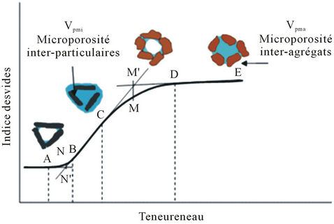
Figure 2. Representation of the soil structure evolution at the desaturation state.
air when water still leaves the porous systems; the aggregates and the particles are connected to each other (shrinkage phase E-C B-O). In the shrinkage curve, the zones which cover these two stages are the curvilinear part (CD & BA).
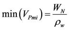
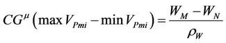
Points M and N represent the water contents at the intersections points of the tangents of the shrinkage curve quasi-linear parts. These parameters are important characteristics for the porous system, because they allow to calculate the minimal and maximum volume of microporosity, and the swelling capacity (“Capacité de Gonflement”, CG) of the porous system according to the following equations (Braudeau et al., 2006):
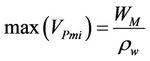
where ,
,  are respectively the moisture ratio at points M and N, and
  is the density of water.
At the particles scale, the swelling capacity can be defined as a micro swelling capacity :
:
where ,
,  are respectively the minimal and the maximal volume of the microporosity.
At the aggregates scale, the macro swelling capacity (CG) is:

where  is the slope of the normal shrinkage phase.
It should be noted that the sample size influences the shrinkage curve slope. Indeed, the smaller the clay sample, the more important the shrinkage curve slope is. That can be explained by the fact that the more important the volume considered is, the higher the existence of macroporosity. So this needs a great quantity of water before reaching its saturation line.
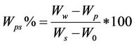
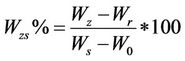
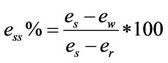
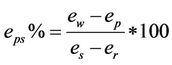
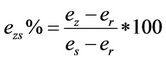
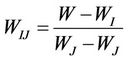
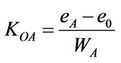
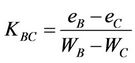
According to [8], the author proposes to use the end points of the differently characterized shrinkage phases to express them as a percentage in relation to the total shrinkage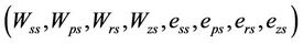 , according to the changes in moisture ratio and void ratio during the drying process. The equations allowing to calculate this percentages are:
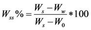
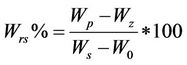
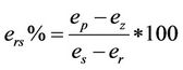
 : the maximum curvature point at the wet side of the shrinkage curve;
 : the transition point from the normal to the residual shrinkage (can be defined by the intersection of the two phases tangents);
 : the transition point from the residual to the zero shrinkage ( can be defined by the intersection of the two phases tangents);
 : the residual shrinkage point, which represents the limit of the shrinkage curve on the dry side.
 : the saturation point.
In Figure 3, we propose a description of the structural evolution taking place in the soil’s skeleton during the saturation and the desaturation phases, as well as an estimation of the different types of water present in the soil.
2.2. The Existing Models Allowing to Describe the Shrinkage Curve
In the literature, several models were proposed to describe the shrinkage curve that can be represented experimentally. The models presented here describe the
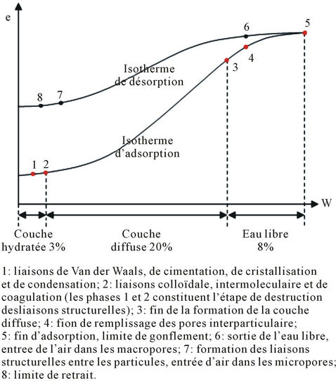
Figure 3. Hydro-structural evolution of an argilo-expansive soil.
relationship between the water content and the void ratio [9].
2.2.1. The Model of Giraldez et al. (1983)
The authors [10] used a third order polynomial function to describe the relation between the void ratio e and the water content W. This model is only valid to describe the zero, residual and normal shrinkage stages of the shrinkage curve by using two parameters.
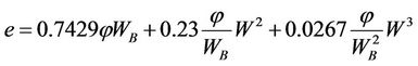
where  is the moisture ratio at the air entry and φ is the slope of the saturation line.
2.2.2. The Model of McGarry and Malafant (1987)
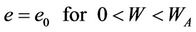
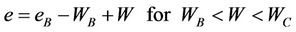
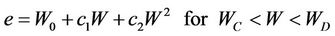
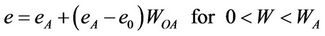
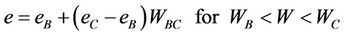
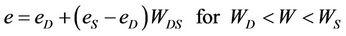
The authors proposed to use linear functions to describe the three distinct stages of the shrinkage curves: residual, normal and structural shrinkage. Using the relationship given by Newman et al. (1979).
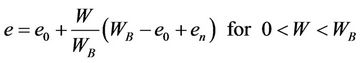
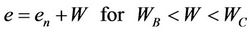
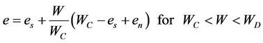
where  is the moisture ratio at the air entry;
  is the swelling limit moisture ratio;
  is the maximum moisture ratio;
  is the void ratio at zero moisture ratio;
  is the void ratio at the air entry value;
  is the intercept of the structural shrinkage curve.
2.2.3. The Model of McGarry and Malafant (1987)
McGarry and Malafant (1987) proposed a generalized model for the S shape shrinkage curves by using four parameters. This model is able to describe the fourth parts of the shrinkage curve:
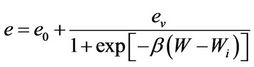
where  is the maximum void ratio range, equal to the void ratio at the saturation
  minus the void ratio at oven dryness
 ; β is a slope parameter depending on the air entry value and
  is the moisture ratio at the inflection point.
2.2.4. The Model of Kim et al. (1992)
Kim et al. (1992) combined an exponential and linear function which gave the best fits to their data by using three parameters.
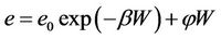
where  is the void ratio at zero moisture ratio; β is a slope parameter depending on the air entry value;
  is the slope of the saturation line.
This model does not consider structural shrinkage, and it represents the normal shrinkage by a linear function, and the zero and residual shrinkage by a reverse exponential function.
2.2.5. The Model of Tariq and Durnford (1993b)
Tariq and Durnford (1993) extended the model of McGarry et al. (1987) by using seven parameters to describe the fourth parts of the shrinkage curve:

where the coefficients, as derived from the boundary conditions, are defined as:


and  and
and  are the void ratio at respectively air entry (in the intra-aggregate pores) and the swelling limit.
2.2.6. The Model of Olsen and Haugen (1998)
Olsen and Haugen (1998) proposed a second order hyperbolic equation, using in its positive solution to describe the shrinkage curve between the zero and the normal shrinkage, and its negative solution to describe the shrinkage curve from normal to structural shrinkage. This model contains six parameters.
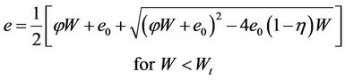
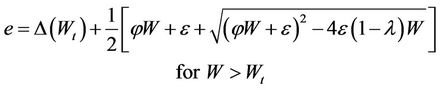
where  reflects the curvature at the transition zones between residual and normal shrinkage,
  reflects curvature at the transition zones between normal and structural shrinkage;
  is a coefficient depending on the upper asymptote;
  is the moisture ratio where the two domains of the shrinkage curve join.
2.2.7. The Model of Braudeau et al. (1999)
Braudeau et al. suggested a seven-parameter-model similar to the Tariq and Durnford (1993b) model. They divided the structural zone into a linear and curvilinear zone, including a point of friability:


where
The slopes of the linear curves are:

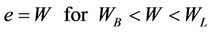
2.2.8. The Model of Chertkov (2000, 2003)
The author proposed an expression based on the statistical analogy between crack networks and the probabilistic microstructure of a matrix consisting only of clay particles:

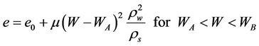
μ is a model coefficient;  is the density of water;
  is the density of the solid particles;
  is the liquid limit, which is the maximum moisture ratio in the solid state of the clay, or at which the shear strength approaches that of a liquid.
3. Material and Method
To reproduce the soil’s shrinkage curve experimentally, we must measure the change of the volume and the weight during all the test process simultaneously. To perform this experiment, we use the measurement device basically used to carry out the desiccation test according to [11] (Figure 4).
This measurement device is usually used to measure the axial deformation during the drying process, but in our study we use it to measure the axial deformation in both wetting and drying processes. The intact sample submitted for testing was a clayey soil with a little carbonate nodules (7%) from the village of Moulay el Bergui near the city of Safi (Morocco). The intact samples were taken from 1.8 - 2.4 m depth.
The tests were performed as follows:
At first, undisturbed samples were taken from field using a sampling box, in the view to preserve the initial structure of the soil. Then, test tubes of 3.6 cm diameter were carefully cut from the undisturbed bloc, and placed in the testing apparatus. Once the test tube was fixed in the receptacle, we place all the mechanism over a balance in order to measure the weight and the volume change both at the same time. After a first reading at its natural state, we begin supplying water by stages (2 g of water at each stage) and at each stage the weight and the axial deformation were taken after the stabilization of the axial deformation. During the wetting process, we protected the upper plane of the test tube by a thin plastic film to avoid water evaporation, and all the mechanism was placed in a box whose the temperature and the humidity were controlled.
After saturation and total stabilization of the axial deformations, we begin the drying process. We start to take measurements along the free air dehydration, then when the axial deformations were stabilized, we place the sample in the oven (105˚C) for 72 hours, taking its weight and deformations values every 6 hours.
The temperature of the testing room was 20˚C and its humidity was 50%.
4. The Shrinkage Curve Modeling
In our testing approach, we study the unidimensional
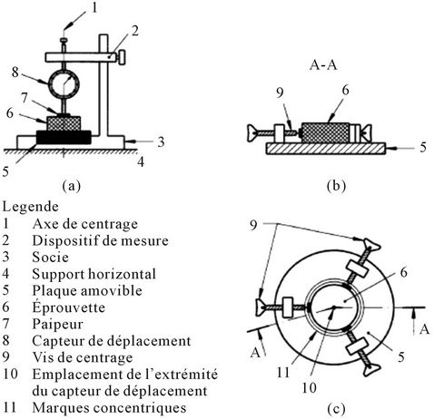
Figure 4. Measurement device of the volume’s changes. (a) Le bâti; (b) Plaque amovible vue en coupe; (c) Plaque amovible vue de dessue.
volume variation of three test-tubes, considering that the tested soil is non-rigid and homogeneous and that there is no shearing between the soil particles. The choice of the physical parameters for our model was based on the fact that the value of the soil’s deformation is the result of the spacing between the particles following the thickness variations of the diffuses layer. This is the variation of the void ratio according to the water content of the medium.
The shrinkage curve model integrates only intrinsic physical parameters of the soil, and the model is described by a third degree polynomial equation as follow:
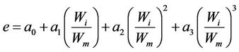 (1)
(1)
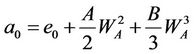
The values  will be deduced from the boundary conditions of the process as follow:
When the soil is dry:  so
so 
When the soil is saturated:  so
so 
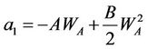
By derivation of the Equation (1):
 (2)
(2)
When the soil is dry: ,
,  so
so 
When the soil is saturated:  so
so 
We obtains the Equation (3) as follow:
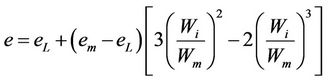 (3)
(3)
Because the results obtained by the Equation (3) was not too accurate, we opted for a new water coefficient, where we deduced the shrinkage limit from both the maximal water content and the considered water content as follows (changing  by
by )The analytical model of the soil’s behavior during the desaturation phase:
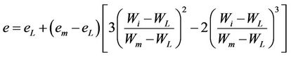 (4)
(4)
where  is the void ratio at the shrinkage limit;
  is the maximal void ration in a saturated state;
  is the maximal water content, and
  is the shrinkage limit.
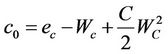
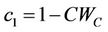
We also try to adapt this model to the saturation curve, according to the following formulation:
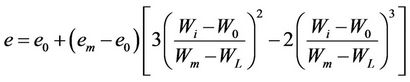 (5)
(5)
where  is the natural water content.
5. Results and Discussion
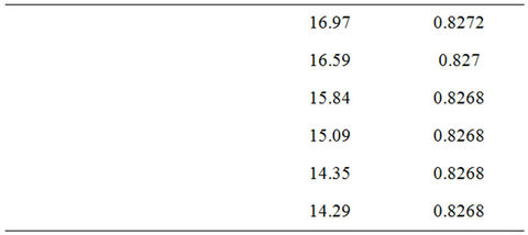
The experimental data and the corresponding soil’s shrinkage curve are represented in Tables 1(a) and (b) and Figure 5. Note that the data represented below are the average of three tests conducted on the same clayey soil.
For the desaturation curve, we observe that the measured shrinkage of the samples cover practically the complete water content range, from the shrinkage curve’s wet side to its dry one.
The comparison between the shrinkage curve experimentally performed and the one calculated by the previous model shows a good correlation between the two methods, and proves that this model is functional for this type of soil. The advantages of this model during the desorption process are:
• The use of a single equation which covers all the phases of the shrinkage curve;
• A reduced number of physical parameters;
• A good correlation between the analytical and the experimental results during the drying process.
In addition, we try to evaluate the adsorption curve for the same soil with the same model, except that we change  by
by . For the adsorption curve, the model does not follow the experimental curve perfectly; it did not give a perfect correlation between the experimental results and the analytical model.
6. Conclusion
The current paper proposes a new model of the shrinkage curve on the basis of the soil’s water content and its structural evolution. This current model is able to cover
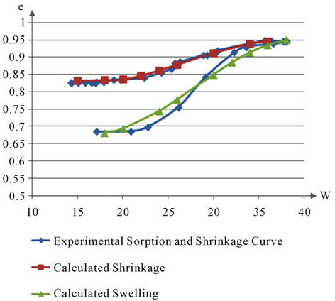
Figure 5. Curve of adsorption and desorption of undisturbed clay samples.
 (a)
(a)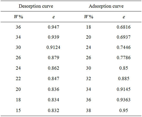 (b)
(b)
Table 1. (a) Experimental results of water content and void ratio variations; (b) Calculated results of water content and void ratio variations.
the fourth parts of the shrinkage curve (structural, normal, residual and zero shrinkage) by using only a third degree polynomial equation according to the limits of its hydro-structural boundaries. For the testing undisturbed soil, the comparison between the experimental tests and the analytical model gives a good correlation between the two methods during the drying process.
In addition, we try to evaluate the adsorption curve for the same soil with the same model, except that we changed  by
by , but it did not give a perfect correlation between the experimental results and the analytical model.
7. Acknowledgements
This work is part of a research project “Clay Soil Behavior during the Drying Process”, conducted in collaboration by the “Centre Expérimental des Sol-Laboratoire Public d’Essais et d’Etudes” (CES-LPEE) CasablancaMaroc and “Ecole Mohammadia des Ingénieurs” (EMIUM5) Rabat-Maroc.
REFERENCES
- J. J. B. Bronswijk, “Drying, Cracking and Subsidence of a Clay Soil in a Lysimeter,” Soil Science, Vol. 152, No. 2, 1991, pp. 92-99. doi:10.1097/00010694-199108000-00005
- P. H. Groenevelt and C. D. Grant, “Re-Evaluation of the Structural Properties of Some British Swelling Soils,” European Journal of Soil Science, Vol. 52, No. 3, 2001, pp. 469-477.
- D. J. Kim, H. Vereecken, J. Feyen, D. Boels and J. J. B. Bronswijk, “On the Characterization of the Unripe Marine Clay Soil. 1. Shrinkage Processes of an Unripe Marine Clay Soil in Relation to Physical Ripening,” Soil Science, Vol. 153, No. 6, 1992, pp. 471-481.
- A. R. Tariq and D. S. Durnford, “Analytical Volume Change Model for Swelling Clay Soils,” Soil Science Society of America Journal, Vol. 57, No. 5, 1993, pp. 1183-1187.
- E. Braudeau, J. M. Costantini, G. Bellier and H. Colleuille, “New Device and Method for Soil Shrinkage Curve Measurement and Characterization,” Soil Science Society of America Journal, Vol. 63, No. 3, 1999, pp. 525-535.
- D. McGarry and K. W. Malafant, “The Analysis of Volume Change in Unconfined Units of Soil,” Soil Science Society of America Journal, Vol. 51, 1987, pp. 290-297.
- E. Braudeau, J. P. Frangi and R. H. Mohtar, “Characterizing Nonrigid Aggregated Soil-Water Medium Using Its Shrinkage Curve,” Soil Science Society of America Journal, Vol. 68, 2004, pp. 359-370.
- X. Peng and R. Horn, “Modeling Soil Shrinkage Curve across a Wide Range of Soil Types,” Soil Science Society of America Journal, Vol. 69, 2005, pp. 584-592. doi:10.2136/sssaj2004.0146
- W. M. Cornelis, J. Corluy, H. Medina, J. Díaz, R. Hartmann, M. Van Meirvenne and M. E. Ruiz, “Measuring and Modelling the Soil Shrinkage Characteristic Curve,” Geoderma, Vol. 137, No. 1, 2006, pp. 179-191.
- J. V. Giraldez, G. Sposito and C. Delgado, “A General Soil Volume Change Equation: I. The Two-Parameter Model,” Soil Science Society of America Journal, Vol. 47, No. 3, 1983, pp. 419-422.
- French Standard XP_P94-060-2, “Drying Test. Part 2: Effective Determination of the Shrinkage Limit on an Undisturbed Sample,” 1997.