American Journal of Climate Change
Vol.2 No.2(2013), Article ID:33518,18 pages DOI:10.4236/ajcc.2013.22015
Consistency of Hydrologic Relationships of a Paired Watershed Approach
1College of Engineering, University of Georgia, Athens, USA
2Center for Forested Wetlands Research, US Department of Agriculture-Forest Service, Cordesville, USA
3Biological and Agricultural Engineering, North Carolina State University, Raleigh, USA
4Weyerhaeuser Company, Columbus, USA
Email: seganeh@uga.edu
Copyright © 2013 H. Ssegane et al. This is an open access article distributed under the Creative Commons Attribution License, which permits unrestricted use, distribution, and reproduction in any medium, provided the original work is properly cited.
Received December 7, 2012; revised January 9, 2013; accepted January 19, 2013
Keywords: Drained Pine Forests; Water Table Elevation; Daily Flow; Calibration; Treatment Effects; Bootstrapped Geometric Mean Regression; Recursive Residuals; CUSUMS; Flow Duration Curve
ABSTRACT
Paired watershed studies are used around the world to evaluate and quantify effects of forest and water management practices on hydrology and water quality. The basic concept uses two neighboring watersheds (one as a control and another as a treatment), which are concurrently monitored during calibration (pre-treatment) and post-treatment periods. A statistically significant relationship between the control and treatment watersheds is established during calibration period such that any significant shift detected in the relationship during treatment is attributed to the treatment effects. The approach assumes that there is a consistent, quantifiable, and predictable relationship between watershed response variables. This study tests the hypothesis that the hydrologic relationships between control and treatment watersheds for daily water table elevation (WTE) and daily flow data were similar without any statistically significant difference during two different calibration (1988-1989 and 2007-2008) and treatment periods (1995-1996 and 2009), when the control and treatment watersheds were interchanged. The watersheds are two artificially drained loblolly pine forests (D1: 24.7 ha and D2: 23.6 ha) located in coastal North Carolina. Results depicted significantly similar WTE regression relationships during the two calibration periods but significantly different WTE relationships during the two treatment periods with reversed control and treatment watersheds. Calibration and treatment flow relationships, and the mean treatment effects on WTE and flow, before and after treatment reversal were significantly different (α = 0.05). The study also discusses causes of differences in hydrologic relationships and treatment effects for such reversal of treatments during a 21-year span of the study on these two similar and adjacent watersheds. The observed differences in the hydrologic relationships between control and treatment watersheds before and after treatment reversal may be attributed to climate or hydrologic non-stationarity which may affect the reliability of paired watershed approach especially when the calibration periods are short.
1. Introduction
Much of the existing knowledge and science on effects of forest management and silvicultural practices on water yield, peak flows, and water quality are in great part based on results from experimental watersheds at sites such as Hubbard Brook (New Hampshire), Coweeta Hydrological Laboratory (North Carolina), H. J. Andrews Experimental Forest (Oregon), Rio Grande National Forest (Colorado), and San Dimas National Forest (California) [1]. The experiments used a paired watershed approach to quantify effects of various forest management activities on the above hydrological variables [2-11]. The basic concept of a paired watershed method involves use of two neighboring watersheds (one as a control and another as a treatment), which are concurrently monitored during calibration (pre-treatment) and post-treatment periods [12]. A statistically significant relationship between the control and treatment watersheds is established during calibration period such that any significant shift detected in the relationship during treatment is attributed to the treatment effects. The approach has been extended to other fields of study to assess effectiveness of conservation practices [13-15]; agroforestry [16-20]; nitrogen and phosphorus management [21,22]; riparian restoration
[23]; controlled drainage [24-26]; and land development [27].
Loftis et al. [28] demonstrate advantages of using paired watershed approach compared to single watershed studies. They show that if the correlation coefficient between the responses of the two watersheds is high (r ≥ 0.9), then the required minimum detectable effect is half for paired watershed studies compared to single watershed studies. The minimum detectable effect is defined as the smallest change in the hydrologic response that is statistically significant. They also illustrate that moderate correlation coefficients (r ≥ 0.6) are adequate to detect treatment effects for paired watershed studies. Clausen and Spooner [12] list advantages of paired watershed studies to include statistical control of climatic and hydrological differences between the two watersheds, and the lack of the necessity to monitor all variables causing change. Prokopy et al. [29] extended the above advantages to demonstrate usefulness of the approach in developing social indicators to assess effectiveness of watershed management programs. However, [30] highlight limitations of the paired watershed approach to include concerns over applicability of results to watersheds under different climate or geology, skewed treatment effects due to extreme climatic events during treatment periods, and the lack of a true replication by the approach. Vogl and Lopes [31] use recursive residual analysis to demonstrate how structural changes in watershed climate during treatment may yield erroneous treatment effects. Alila et al. [32] and [33] argue that the use of paired watershed approach to quantify effects of forest management on peak-flows is flawed because the pairing of magnitudes between control and treatment watersheds does not account for changes in the frequency of the magnitudes. They demonstrate that the effects of forest harvesting on peak-flows increase with increase in the return period. Som et al. [34] demonstrate that use of classical ordinary least squares (OLS) approach to detect statistically significant treatment effects may not account for temporal autocorrelation of hydrologic data and thus may give incorrect prediction confidence intervals. Work by [35] highlights the limitation of the approach to quantifying effects of urbanization on components of the hydrologic cycle. The above concerns over the paired watershed approach have inspired use of hydrologic models to assess effects of climate and land use change on watershed hydrology [36-39]. Although hydrologic models are cost and time savers, their relatively higher learning curve and their requirement for multiple data inputs provide challenges to water managers. Also, hydrologic models still require observed data to optimize the model parameters, a process known as model calibration.
Paired watershed comparisons still represent the simplest form of a randomized block design, the most relevant method for water quality monitoring [40]. The combination of a treated and a control watershed forms one un-replicated block. An alternate approach to true replication is to complete a second manipulation which largely duplicates the first but adds some subtle differences in experimental treatment [40]. Schleppi [41] comments that paired watershed studies are still useful in assessing environmental changes at spatial scales with many interactions. For example, [42] use a paired watershed approach to demonstrate how management practices that do not convert forest types are not as significantly affected by extreme climate as practices that do. Also, paired watershed approach provides a feasible methodology for quantifying watershed hydrological effects of shifting from ecosystems of pine forests with natural understory to ecosystems that intercrop pine forests with switchgrass. This shift in ecosystem composition is due to projected environmental benefits of cellulosic biofuel crops such as switchgrass (Panicum virgatum) in contrast to conventional biofuel crops such as corn.
The paired watershed approach does not require the two watersheds to be identical, but comparable in size, topography, vegetation, soils, and climate. However, it assumes that there is a consistent, quantifiable, and predictable relationship between watershed response variables (Flow, water table elevation, soil moisture, evapotranspiration, and nutrients) of the control and treatment watersheds during calibration and treatment [12]. This study tests this hypothesis on relationships between control and treatment watersheds for daily water table elevation and daily flow data during two different calibration and two different treatment periods for statistical difference. During the first calibration period (1988-1989), D1 was under control and D2 was under treatment; both watersheds had a 14-year old pine stand (Table 1). Watershed D2 was harvested (clear-cut) in 1995 and thus a post-treatment period of 1995-1996. D2 was planted in 1997 and by 2004 water table elevations had approximately returned to elevations observed in 1988 [43]. A new study initiated to examine impacts of switchgrass and its intercropping with pine on these watersheds required harvesting (clear-cutting) of the 35-year pine stand on the control watershed (D1) by April of 2009. Thus it provided an opportunity to use the data collected prior to April of 2009 as the new calibration period with D2 (12 years old stand) as the new control and D1 (35 year stand) as the new treatment. This is referred to as reversal of treatment. The data collected from April 2009 to December 2009 before planting of new pine represents the second harvest-treatment. These unique experiments on reversal of treatments are rarely done in hydrologic studies on a watershed scale because of limited study sites, time, and resources yet provide the closest case of replication of paired watersheds. The scientific question
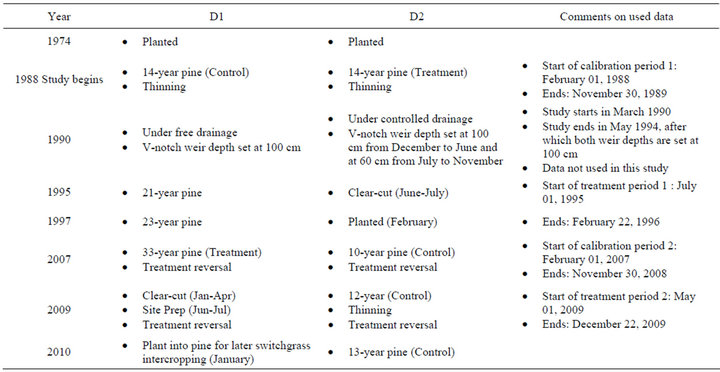
Table 1. Chronology of major operational silvicultural practices on artificially drained, loblolly pine-forested watersheds D1 and D2 from 1974 to 2010. Treatment periods before and after treatment reversal were selected to end before planting.
this study addresses is whether the hydrologic relationships and treatment effects during the first calibration and treatment periods, remain the same in the second calibration and treatment periods where similar watersheds were interchanged for treatment.
Therefore, the first objective of the study is to assess whether the control and treatment daily water table elevation (WTE) and daily flow relationships are statisticcally consistent during the two calibration periods and during the two treatment periods. We hypothesized that by 2007, 13 years after 1995 harvest-treatment on D2, the watershed hydrologic behavior of D2 had reverted to 1988 baseline levels. The assumption was based on synthesis of literature on hydrologic recovery (annual flows) of non-intensively managed forest paired watershed studies. For example, a review of hydrologic recovery on three watersheds in Northeastern US (Fernow 7, Leading Ridge 2, and Hubbard Brook 2) by [2] demonstrated that it took 7 to 25 years for the annual water yields to return to pre-harvesting volumes. The difference in hydrologic recovery rate was attributed to difference in the percent composition of tree species that re-grew after 100% clear-cutting (e.g., conversion of pre-treatment hardwood to post-treatment coniferous). Additional review of the original work by [44] showed that the prolonged hydrologic recovery on the above three watersheds was due to application of herbicides to control natural regrowth. For watersheds where natural regrowth was not controlled (Hubbard Brook Catchments 4 and 5), pre-treatment annual water yields were attained within 3 to 4 years after harvesting [44,45].
The second objective is to examine whether the treatment effects before and after reversal of control and treatment watersheds were significantly different. The operating assumption was that the paired watershed approach is robust to account for any differences in the WTE and flow relationships between control and treatment watersheds during the two calibration and two treatment periods. Approaches to account for differences in treatment effects due to choice of control and treatment watersheds are beyond the scope of this study. Also, the flow duration curves (FDCs) of each watershed are generated to provide insight into differences in hydrologic behavior during the respective calibration and treatment periods with emphasis on slope of the flow duration curve (indicative of extent of flow variability) and shifts in point of cease to flow (indicative of watershed storage).
2. Methods
2.1. Site Description
The study site is on Carteret 7 tract, located in Carteret County, North Carolina (Latitude of 34.822˚ and Longitude of −76.668˚), under the ownership and management of Weyerhaeuser Company. The site consists of three artificially drained experimental watersheds (Figure 1: D1, D2, and D3) that are about 26.31, 25.90, and 27.11 ha, respectively. A fourth watershed (D0) has been recently established north of D1 (Figure 1), for future
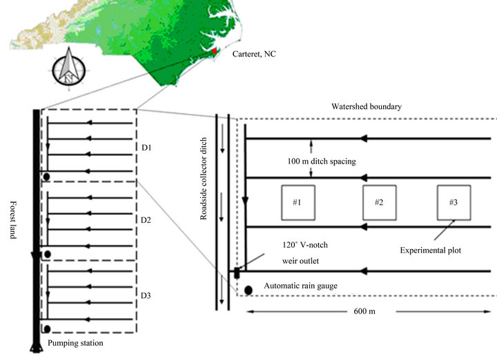
Figure 1. Location and layout of artificially drained pine-forest experimental watersheds with monitoring stations, Carteret County, North Carolina (Adapted from Amatya and Skaggs, 2011). The water table elevation (WTE) is monitored in plots #1 and #3.
studies. The watersheds are surrounded by forested land in the north, south, and west, and by agricultural land in the east. The boundary roads hydrologically separate the watersheds from influences of activities on neighboring lands, while raised beds (≈0.4 m) minimize surface flow between watersheds [26]. McCarthy et al. [46] characterized the topography of the site as flat Coastal Plain with a gradient of 0.1% and ground surface at about 3 m above sea level. The Deloss fine sandy loam soil on the site is classified as very poorly drained with a shallow water table under natural conditions. Each watershed is drained by four parallel lateral ditches about 1.4 - 1.8 m deep, spaced 100 m apart (Figure 1). The mean annual rainfall over a 21-year period is 1517 mm with a 10% - 15% annual increase due to hurricanes and tropical storms [47]. The simulated annual Penman-Monteith potential evapotranspiration (P-M PET) using leaf area index and stomatal conductance ranges from 978 mm to 1334 mm [47]. The P-M PET simulations are based on DRAINMOD-FOREST developed by [38]. For a detailed description of the site soil parameters, climatological data, and forest vegetation, the readers are referred elsewhere [26,38,46,47].
2.2. Data Collection
The three experimental watersheds (Figure 1) were instrumented in 1988 to measure and record drainage rate, water table depth, water quality, rainfall and meteorological data. Total rainfall is collected with two automatic tipping bucket rain gauges backed up by a manual gauge in an open area. Air and soil temperatures, relative humidity, wind speed, solar and net radiation are currently collected on 15 minute interval using a Campbell Scientific CR10X full weather station installed in a 10- foot tower located in an open area near watershed D3. An adjustable height 120˚ V-notched weir, located at the outlet of each watershed, facilitates measurement of drainage outflow by continuously recording water levels upstream of the weir where the bottom of the V-notch is about 100 cm below average soil surface elevation for each watershed. The V-notch weir has an automatic stage recorder set in a water level control structure at a depth of 0.3 m from bottom of outlet ditch to make measurements every 12 minutes. A pump was installed in 1991 at the roadside collector ditch outlet downstream of all watersheds to minimize weir submergence during large events [26].
Flow was computed using discharge-stage relationships for non-submerged and submerged weir conditions [48]. Calculated daily flow values greater than the capacity of the downstream culvert were capped to 45 mm/day; the approximate drainage capacity [47]. Such data were excluded from analysis of treatment effects because under fully saturated conditions when water table elevation is at or near the surface, the flows are likely the same in both watersheds, and therefore treatments effects are insignificant. Also, the computed flow data during high weir submergence are susceptible to high uncertainty. Water table elevation (WTE) is continuously recorded at the front and back experimental plots (Figure 1) of each watershed. The average of the back and front WTE is the representative WTE for each watershed. For this study only data collected on D1 and D2 are used for comparing treatment effects before and after reversal of control and treatment watersheds.
2.3. Study Design and Treatments
A paired watershed approach [12,28] was used to test the consistency of relationships between daily water table elevation and daily flow for D1 and D2 watersheds during two independent calibration and two independent treatment periods. Table 1 presents the chronology of major silvicultural treatments on D1 and D2 watersheds between 1988 and 2010. The treatment periods were selected to span the same period after harvesting (clearcutting) and to end before planting of young pines on the treated watersheds. The first calibration-treatment periods consist of watershed D1 as the control while D2, which was harvested in 1995, as the treatment watershed. Both watersheds were under 14 to15-year old pine stands at the start of the calibration period (1988) when free drainage at three different weir depths of 60 cm, 80 cm, and 100 cm below the ground surface elevation (GSE), was tested. However, watershed D2 underwent controlled drainage (weir depth set at 60 cm below GSE) from 1990 between June and November of each year while D1 was at 100 cm depth, until it was harvested in 1995. By 1995, all weir outlets were again set at a depth of 100 cm. Therefore, daily data for the first calibration period spanned the period of February 01, 1988 to November 30, 1989. Watershed D2 was completely harvested by July of 1995. Therefore, July 01, 1995 to February 22, 1996 formed the first harvest-treatment period. Only data where the weir depth was set at 100 cm is used to maintain consistency across the two different calibration periods.
The second calibration-treatment periods consist of treatment reversal, where watershed D1 that had been the control since 1988 was completely harvested in April of 2009, when it was a 35 years old pine stand following Weyerhaeuser’s operational practice. At the time of this harvesting, watershed D2 had a 12-year old pine stand that had regenerated after planting in 1997. Thus, for the reversal of the harvest-treatment period, watershed D2 became the control while D1 became the treatment. Because harvesting of D1 started in December 2008, Water table elevation and flow data from the two watersheds from February 01, 2007 to November 30, 2008 were used for the second calibration. Although, the stand age of the treatment watershed D1 was about 33 - 34 years, this period was chosen because the stand age (12-year old pine) on the new control watershed (D2) was closer to the stand age at the beginning of the first calibration period (14 to 15-year old pine stand). Also, [49] showed that the WTE of the treatment watershed D2 returned to the baseline levels of 1988-1990 by the end of 2004. Harvesting of the new treatment watershed (D1) was completed by April, 2009; therefore, May 01, 2009 to December 22, 2009 formed the period for replication of treatment effects after treatment reversal. The type of treatment considered in this study is the combined effect of pine harvesting and, shearing and bedding (operational practice before replanting) on daily WTE and daily flow.
2.4. Preliminary Analysis
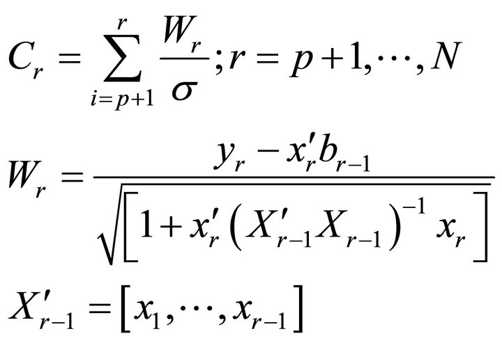
The cumulative sum of squared recursive residuals test (CUSUMS; [50]) was used to test whether there were structural changes in the data for developing regression equations of the two calibrations and two treatment periods. The CUSUMS test enables the assessment of existence of external effects on the watersheds other than treatment effects by examining the stability of the regression coefficients during the respective calibration and treatment periods. The CUSUMS test assumes that the variability of the cumulative sums of the recursive residuals follow a Brownian motion with an expected mean of zero and a variance equal to the total degrees of freedom of the regression model. According to [50], the mathematical formulations of recursive residuals are defined by Equation (1). Recursive residuals in contrast to ordinary least-squares (OLS) residuals for diagnostic statistics of regression equations are: identically and independently distributed; not constrained to sum to zero; and provide a mechanism for detection of change in the regime of the regression equation [50,51].
 (1)
(1)
where Cr is the rth cumulative sum of recursive residualsp is the total number of regression coefficients, N is the total number of data samples, Wr is the rth recursive residual, yr is the rth observation of the response variable, xr is the rth column vector of the explanatory variables ( is the corresponding row vector), br−1 is the ordinary least squares estimate of parameter b using all data before the rth sequential data point, and σ2 is the variance of the recursive residuals.
Recursive residuals and the plots of squared recursive residuals were computed using an econometric toolbox developed by [52]. Structural changes or instability of regression coefficients are detected if the cumulative sums of squared recursive residuals exceed the critical bounds at a 5% level of significance (bounds of the 95% confidence interval).
2.5. Paired Watershed Approach
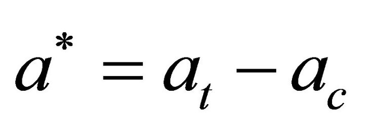
The treatment effects on the water table elevation for each pair of calibration-treatment data were quantified using mathematical formulations of a paired watershed approach by [28]. Given calibration equation [Equation (2)] and the treatment equation [Equation (3)], the treatment adjustment to the intercept and slope were computed by Equations (4) and (5). Then, the treatment effects were computed using Equation (6).
 (2)
(2)
 (3)
(3)
 (4)
(4)
 (5)
(5)
 (6)
(6)
where Yc and Yt are the hydrologic responses from the treatment watershed during calibration and treatment periods, respectively; Xc and Xt are the responses from the control watershed during calibration and treatment, respectively; ac and at are the linear regression intercepts for calibration and treatment, respectively; bc and bt are the linear regression slopes for calibration and treatment, respectively; a* and b* are the treatment adjustment to the intercept and slope, respectively; Yte is the cumulative effect for the treatment period under consideration; and Xcm is the mean of the response from the control watershed during the treatment period.
 (7)
(7)
Preliminary analysis gave similar treatment effects using a dummy variable T for treatment, to fit a single equation [Equation (7)] for both treatment and control data. The dummy variable was set to zero during the calibration period and set to one during the treatment period. The coefficient γ corresponds to the treatment effects. The above two approaches gave similar treatment effects as the mean of the differences between the observed and expected responses (traditional approach) during the treatment period. A paired t-test statistic and 95% confidence intervals of mean treatment effects were used to evaluate whether the treatment effects before and after treatment reversal were significantly different for daily WTE and daily flow. The t-test analysis was based on differences between observed and expected responses of the treatment watershed during the respective treatment periods. Similar analysis was implemented for the daily flow relationships.
2.6. Bootstrap Geometric Mean Regression
The intercept and slope of the linear relationships [Equations (2) and (3)], and their respective 95% confidence intervals were estimated by bootstrap geometric mean regression, also known as the bootstrap reduced major axis regression [53]. Bootstrapping resamples a single dataset a predefined number of times with replacement, such that subsequent statistics and regression coefficients are determined from the bootstrap sample. While geometric mean regression first determines the slope of linear regression line by transforming the response and explanatory variables to have a mean of zero and a standard deviation of one. The resultant slope is referred to as the geometric mean of the linear regression of the response on the explanatory variable [54]. This study used a nonparametric bootstrap resampling approach and computed the 95% confidence intervals based on assumption of asymmetric F-distribution of the estimator [55]. One thousand bootstrap samples were used to compute for the regression coefficients and for the corresponding confidence intervals.
2.7. Flow Duration Curves
The flow duration curves (FDCs) for each watershed during each period were generated using the Weibull plotting position [56] expressed by Equation (8). Where P is the probability of exceedence, r is the rank of specific flow based on the data record, and n is the size of the data under consideration.
 (8)
(8)
3. Results and Discussion
3.1. Calibration and Treatment Data
Daily water table elevation (WTE) and daily flow during the two calibration (02/01/1988 to 11/30/1989 and 02/01/2007 to 11/30/2008) and two treatment (07/01/ 1995 to 02/22/1996 and 05/01/2009 to 12/22/2009) periods are presented in Figures 2 and 3, and the corresponding statistics in Table 2. Figure 2 demonstrates the seasonal effect on WTE and flow, such that the WTE drops below 1.5 m (above sea level) in the summer with occasional events that temporarily raise the water table. For both calibration periods, the lowest WTE is recorded in July of the first year when the weir depth in both cases was set at 100 cm below the average surface elevation (2.75 m). The average WTE on D1 is higher than WTE on D2 for both calibration periods (Figure 2). This is reflected by a consistent difference of about 5 cm between WTE of D1 and D2. Use of a paired t-test to assess the mean difference of daily WTE between D1 and D2 (D1-D2) during the two calibration periods showed no statistically significant difference at 5% level of significance. The above statistical test affirms the supposition that by 2007, the hydrologic response of the WTE on D1 and D2 had definitely returned to 1988 levels. Earlier analysis by [49] report that by 2004, the WTE for both watersheds had returned to 1988 levels. The figures also illustrate the dependency of daily flow on WTE because most flows coincide with high WTE (WTE > 2.0 m).
Figure 3 shows the expected increase in WTE due to treatment (clear-cutting). For both treatment periods, the watershed under treatment (D2 during period 1 and D1 during period 2) shows elevated WTE in contrast to WTE of watershed under control. The elevated levels are visually higher than base levels during the calibration
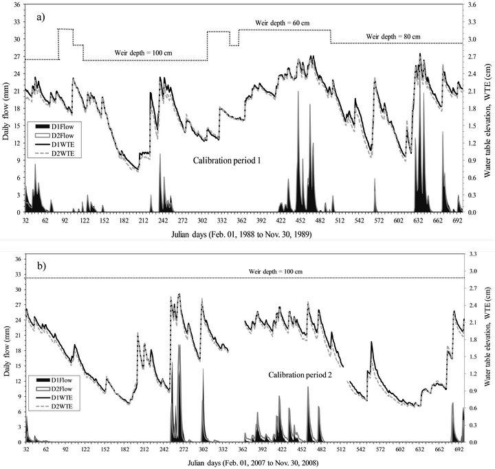
Figure 2. Comparison of daily water table elevation, WTE (m) and daily flow (mm) for watersheds D1 and D2 during two calibration periods. During the first calibration period (1988 to 1989; Figure 2(a)), the weir depth was set at 60 cm, 80 cm, and 100 cm below the average surface elevation of 2.75 m. However, during the second calibration period (2007 to 2008; Figure 2(b)), weir depth was set at 100 cm. The lines are indicative of WTE trends while area plots are indicative of flow trends.
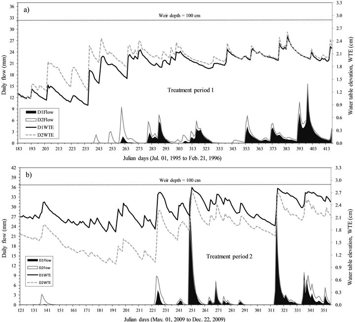
Figure 3. Comparison of daily water table elevation, WTE (m) and daily flow (mm) for watersheds D1 and D2 during two treatment periods. During the first treatment period (1995 to 1996; Figure 3(a)), D1 is under control while D2 is under treatment (clear-cutting) However, during the second treatment period (2009; Figure 3(b)), D2 is under control while D1 undergoes treatment (clear-cutting). The weir depth during the two treatment periods is set at 100 cm. The lines are indicative of WTE trends while area plots are indicative of flow trends.
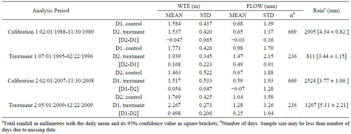
Table 2. Statistics of daily water table elevation (WTE), discharge (FLOW), and total rain.
periods. However, during high-saturation periods (WTE > 2.5 m), the difference in WTE of treatment and control watersheds is not as great as during low-saturation dry periods. The higher difference in WTE at the beginning of both treatment periods is attributed to higher differences in evapotranspiration (ET) rates during the growing season in contrast to ET rates during the dormant season with less ET demands. This is because the pine rooting depths on control watersheds are deeper and therefore, make it possible for pine to access lower WTE to meet the ET demand yet the clear-cut watershed has reduced interception of rain and reduced ET demand. The temporal variation of flow events during the two treatment periods is different. There are more smallevents (flow <9 mm/day) spread out during the six months of treatment period 1 while two large events (flow >20 mm/day) dominate the second treatment period as possibly affected by the rainfall intensity, initiation, and duration during the two different periods.
Inspection of means of daily flow data during the two calibration periods (Table 2) depicts relatively higher flows from D1 during calibration period 1while higher flows from D2 during calibration period 2. The trend is as expected for the first calibration period because average WTE in D1 is relatively higher than average WTE in D2 and both watersheds are under 14 years old pines. However, the trend is counterintuitive during calibration period 2 because, average WTE in D1 is still relatively higher than average WTE in D2. This may be attributed to difference in age of the pine trees (34 year for D1 and 14 years for D2) and that the soils of D2 may not have fully recovered from operational silvicultural practices of harvesting, shearing, and bedding that occurred during and after treatment of 1995. The above practices, specifically bedding affect horizontal flow in the disturbed soil horizons.
Examination of rainfall data (Table 2) shows more rain during the first calibration period (average daily of 4.3 mm) than in the second calibration period (average daily of 3.8 mm). Also, more rain in the second treatment period (average daily of 5.1 mm) compared to the first treatment period (average daily of 3.4 mm). The average daily rainfall during the two calibration periods was not significantly different at 5% level of significance; however, it was significantly different during the two treatment periods (Table 2). The above climatic trends are not reflected in average daily WTE and daily flow. However, the highest variability of WTE is during the second calibration period (second-highest variability in daily rainfall; Table 2), while the highest variability of daily flow is during the second treatment period (the highest variability in daily rainfall).
3.2. Structural Stability of Regression Models
Preliminary analysis using ordinary least squares (OLS)
estimates of linear regression coefficients for WTE showed no significant structural shifts in the simple linear coefficients for 1988 to 1989 calibration data (Figure 4(a)), 1995 to 1996 treatment data (Figure 4(c)), and 2009 treatment data (Figure 4(d)). This was determined by the lack of movement of the cumulative sums of squared recursive residuals (CUSUMS) outside the critical bounds (straight lines, indicative of the 5% level of significance or 95% confidence interval). Thus, there was no evidence of significant structural instability for the linear models during the specified periods.
However, there was a single break point in the 2007 to 2008 calibration data (Figure 4(b)). The estimated structural break point is in the neighborhood of dates with missing data (December 06-30, 2007). Therefore, the break was assumed to be caused by missing data than a major external influence. This assumption was validated by comparing linear regression coefficients using data before the break and all 2007 to 2008 calibration data. The comparison results showed no significant difference (at 5% level of significance) between the regression coefficients of the two datasets. Also, evidence of structural shifts in regression coefficients would be undesirable if observed during the treatment period because then the estimated treatment effects would include external impacts other than the treatment under consideration.
The structural stability of linear models was checked using OLS estimates of regression coefficients, yet the final fitted models were based on bootstrapped geometric mean regression. The two approaches give different coefficients (intercepts are significantly different). The use of OLS was for preliminary analysis because bootstrapped geometric mean regression provided narrow confidence intervals at 5% level of significance for the regression coefficients compared to OLS. Therefore, estimates of the coefficients based on bootstrapped geometric mean regression were considered to be more stable and reliable for subsequent analysis. Similar analyses on the flow data showed no structural instability of the fitted models.
3.3. Fitted Regression Models
3.3.1. Water Table Elevations
Both the intercept and slope of the WTE based on the second calibration period (2007 to 2008; Figure 5(a)), fall within the 95% confidence intervals of the intercept and slope of the WTE for the first calibration period (1988 to 1989). Therefore, the relationships of the WTE between D1 and D2 during the two calibration periods are strong (R2 ≥ 0.98) and consistent, indicating no statistically significant difference (α = 0.05) during the two periods. This affirms earlier discussion that by 2007, the WTE dynamics of D1 and D2 had returned to 1988 baseline levels. The calibration results showed that rainfall

Figure 4. Plots of cumulative sums of squared recursive residuals (CUSUMS) of a linear relationship between water table elevations of control and treatment watersheds. (a) 1988 to 1989 calibration period, (b) 2007 to 2008 calibration period, (c) 1995 to 1996 treatment period (D under control; D2 under treatment), and (d) 2009 treatment period (D2 under control; D1under treatment). Data is based on only days when the weir depth was at 100 cm below the average surface elevation.
amount and difference in age of the pine stands on the paired watersheds did not significantly alter the WTE relationships during the two pre-treatment periods. The average daily rainfall during the first calibration period was 4.3 mm/day and an age difference between control and treatment pine forests of zero (both watersheds with pine stand age of 14 - 15 years), compared to rainfall of 3.8 mm/day and age difference of about 20 years (D2: 11 - 12 years old and D1: 34 - 35 years old) during the second calibration period. One reason may be that the canopy coverage and structure, and thus leaf area index (LAI) on both watersheds with this difference in stand age may be similarly affecting the WTE [57].
The WTE relationships during the two treatment periods are strong (R2 ≥ 0.72) and significant (p < 0.001). However, the intercepts and slopes of the WTE regression equations are significantly different (Figure 5(b)). This is expected because historically (1988-1989) WTE of D1 was consistently higher than WTE of D2. Therefore, clear-cutting of D1 resulted in even higher WTE than clear-cutting of D2. This is demonstrated by a consistently higher regression line due to higher intercept for treatment period 2 than treatment period 1 (Figure 5(b)). Although the WTE relationships are inconsistent (significantly different slopes and intercepts) during the two treatment periods, an hypothesis of similar treatment effects before and after reversal of control and treatment watersheds was tested in subsequent subsections because the paired watershed approach is designed to account for these differences if the treatment effects are the same.
3.3.2. Daily Flow
The daily flow relationships during the two calibration and two treatment periods are significantly different (Figures 6(a) and 6(b)). For both cases of calibration and treatment, the intercepts and slopes are significantly dif-
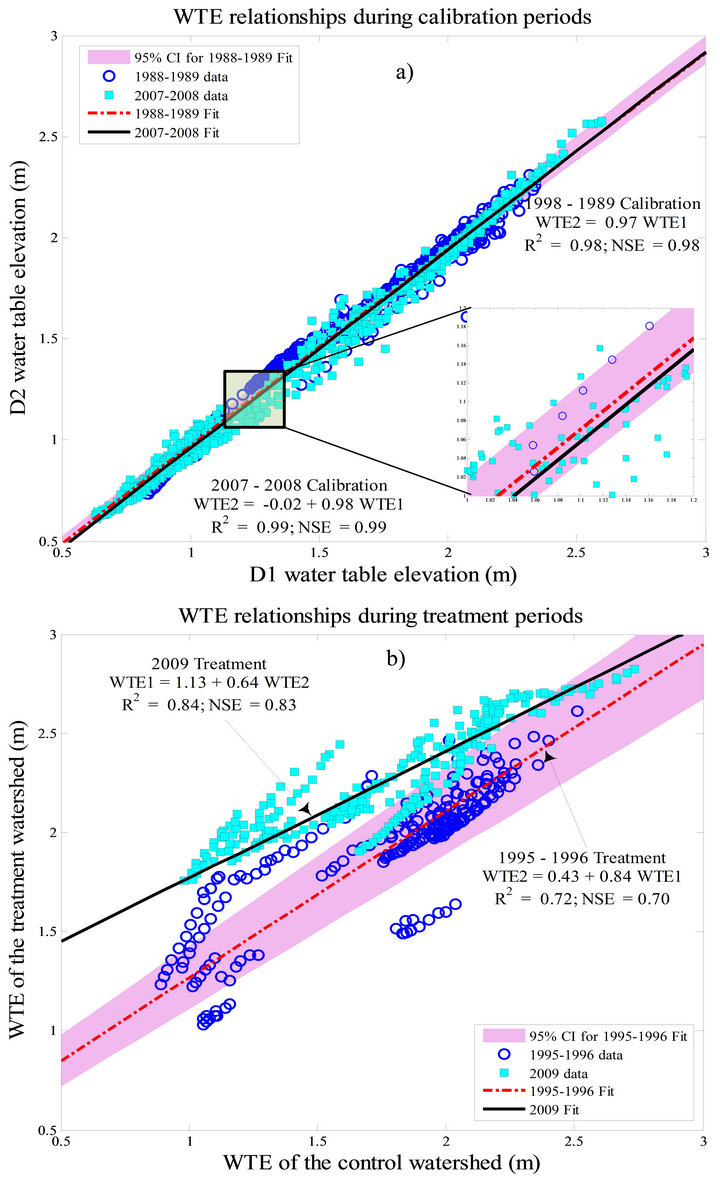
Figure 5. Comparison of daily water table elevation (WTE) relationships between control and treatment watersheds during two calibration periods (Figure 5(a)) and two treatment periods (Figure 5(b)). The 95% confidence band is for the period before reversal of control and treatment watersheds. WTE1 is daily water table elevation for D1 and WTE2 for D2.
ferent. This difference is primarily attributed to modifycation of soil properties of the top layer (0 to 70 cm) during the operational silvicultural activities of shearing and bedding, and soil compaction by machinery during clear-cutting and logging [58-62]. Study by Grace et al. [59] showed that soil compaction during harvesting of hardwoods on poorly drained soils of a Tidewater region of North Carolina increased the soil bulk density by 18.5% (from 0.22 to 0.27 g∙cm−3) and reduced the saturated hydraulic conductivity by 79.3% (from 397 to 82 cm∙hr−1). Rab [62] reports that even 10 years after timber harvesting in Australia, there was a 22% - 68% difference in soil physical properties of harvested compared to undisturbed soils. Therefore, the difference in regression
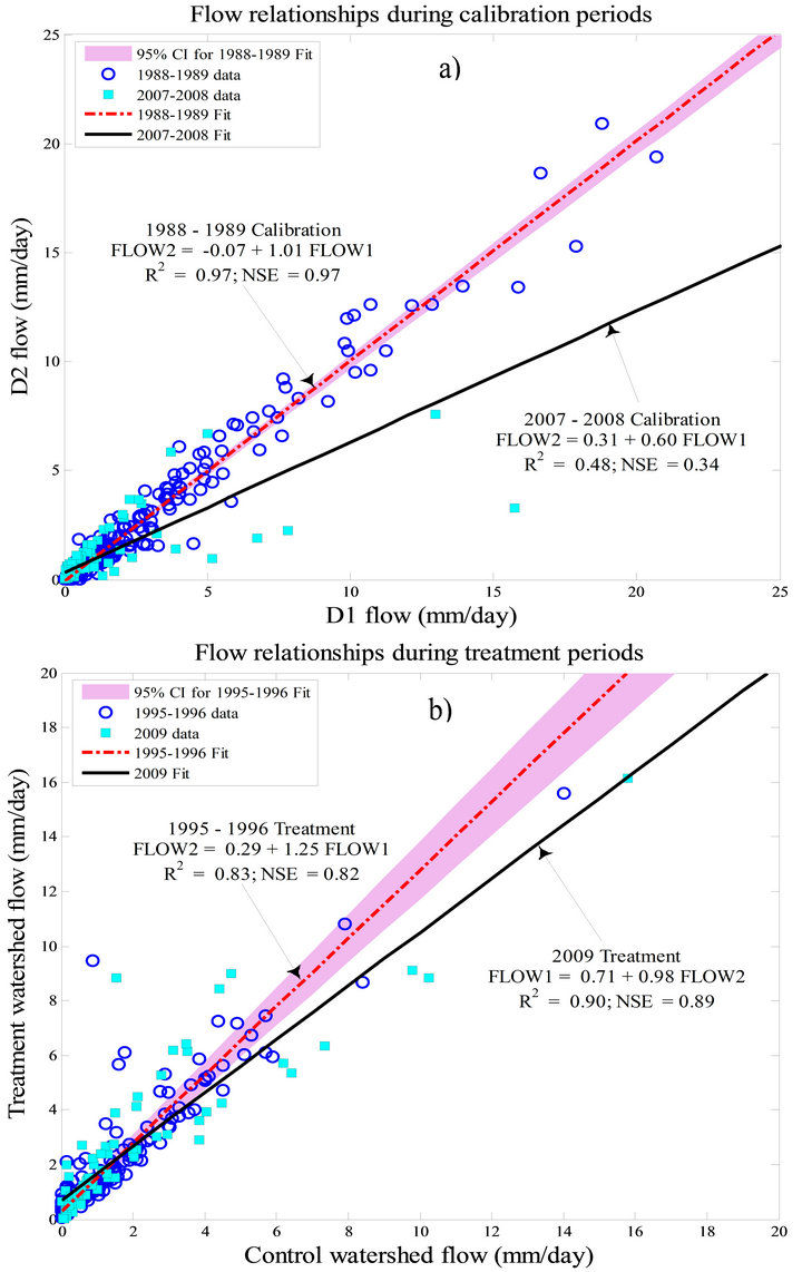
Figure 6. Comparison of daily flow relationships between control and treatment watersheds during two calibration periods (Figure 6(a)) and two treatment periods (Figure 6(b)). The 95% confidence band is for the period before reversal of control and treatment watersheds. FLOW1 is daily flow for D1 and FLOW2 for D2.
relationships of daily flow during the two calibration periods may be attributed to difference in soil properties, especially properties of the top layer (0 - 70 cm), which mostly affects the lateral drainage to the ditches. Also, difference in surface depression storage may have contributed to the observed difference. The surface depresssion storage on a 34 - 35 years old stand is smaller due to settling of beds during that time compared to settling of such beds on 11 - 12 years old stand.
3.4. Treatment Effects
3.4.1. Mean Treatment Effects
The WTE treatment adjustments are positive for the intercepts (Table 3) and negative for the slopes. Thus similar directions of shift in intercept and slope for the two treatment periods. The largest changes both in the slope and intercept of WTE relationships are exhibited in the second treatment period. And thus, the mean treat-
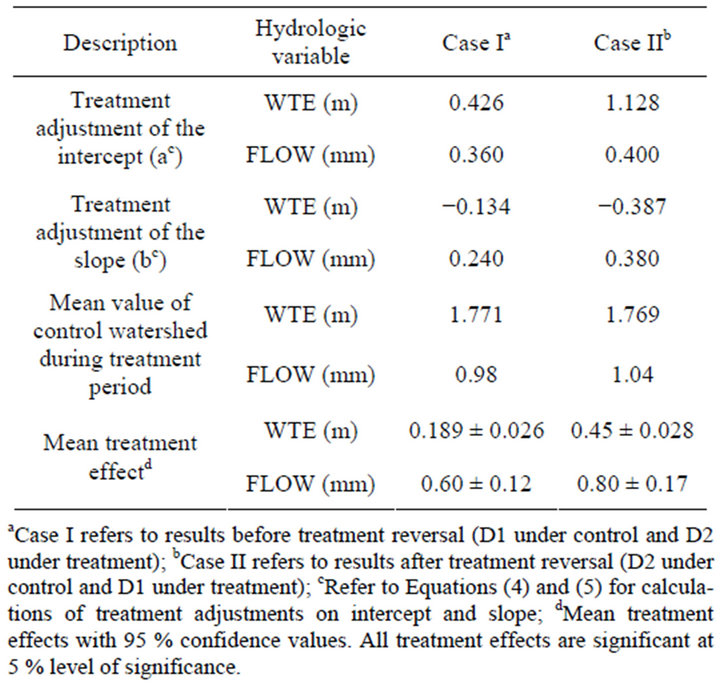
Table 3. Mean treatment effects on the water table elevation (WTE) and flow (FLOW) six months after treatment, before and after reversal of control and treatment watersheds.
ment effect on daily WTE after the reversal of treatment watersheds is greater than the mean treatment effect before the treatment reversal (Table 3). Statistical analysis (paired t-test at α = 0.05) showed significantly different means of treatment effects on WTE before and after reversal of treatments. The 95% confidence interval for each treatment mean shows that all treatment effects are statistically significant (α = 0.05). There was a 138% increase (from 18.9 cm to 45 cm) in the mean treatment effect on WTE after the reversal of the treatments. Although, the average daily rainfall amount was greater during the second treatment period than the first treatment period, one plausible explanation for the increased effect may be attributed to a consistently higher WTE on D1 than D2 such that the paired watershed approach under-estimated the treatment effects when D2 was under treatment and over-estimated the effects when D1 was under treatment. Accounting for the difference in the average rainfall still gives a 59% increase in treatment effect for every millimeter of rainfall during the 2009 treatment period compared to the 1995 to 1996 period. During the first treatment period, for every millimeter of rainfall the treatment effect increased the WTE by 55.6 mm (mean treatment effect of 189 mm/mean rainfall of 3.4 mm) compared to 88.2 mm during the second treatment period (mean treatment effect of 450 mm/mean rainfall of 5.1 mm). The difference in treatment effects may also be attributed to seasonal difference in which the treatment watershed was harvested (clear-cut). The harvest-treatment of 1995 (first treatment period) was in June-July. This is considered to be a dry-weather harvest-treatment, while the 2009 harvest-treatment was in January-April, a winter-spring harvest-treatment (during wet-weather). Several studies report significant differences in treatment effects between wet-weather and dryweather harvest treatments [61,63-65]. Work by [61] demonstrates a 50% difference on elevated WTE between dry-weather (14 cm) and wet-weather (21 cm) harvest-treatment.
Unlike the observed 138% increase in treatment effect on daily WTE due to treatment reversal, the same treatment reversal increased the mean effect on daily flow by 33.3% (from 0.60 mm/d before reversal to 0.80 mm/d after the reversal). Results of a paired t-test (α = 0.05) on differences between expected and observed daily flows on the watershed under treatment before and after the treatment reversal, showed significantly different treatment means. Also, both treatment effects on flow were significant (α = 0.05) as depicted by the respective 95% confidence intervals (Table 3). The daily flow treatment effects before and after reversal of control and treatment watersheds follow the same trend as WTE because WTE is the major driver of flow on these forested coastal watersheds. However, the absolute changes in WTE and flow are different for the two treatment periods. One plausible explanation for this observation may be the difference in temporal distribution of storm events and their initiation during the two treatment periods (Figure 3) and the degree to which they impact WTE and flow. The first treatment period is dominated by small events ( flow ≤9 mm/day) spread across the entire six months, while the second treatment period is dominated by two large events (flow ≥20 mm/day) close to each other (Figure 3). Earlier analysis of rainfall data showed significant different daily means during the two treatment periods (Table 2).
Cumulative treatment effects on WTE before treatment reversal were less than observations of [66] on the Florida cypress-pine Flatwoods but greater after treatment reversal. Sun et al. [66] observed an increase in the WTE of 29 cm after 31 months and a doubling of flow after five months. The difference in treatment effects for the two studies is due to difference in the treatment periods (six months compared to 31 months), difference in the tree species, and difference of soils and climatic conditions at the two study sites. However, the average treatment effects (before and after treatment reversal) for this study are comparable to results of [66]. Also, the results were less than observations of [67] on hydric soils (WTE increase of 48 - 49 cm after 3 months) of Florida Flatwoods landscape but comparable to their observations on nonhydric soils (WTE increase of 19 - 21 cm).
3.4.2. Flow Duration Curves
The flow duration curves (FDCs) of all periods (Figure 7) show that watersheds D1 and D2 have no baseflow be-
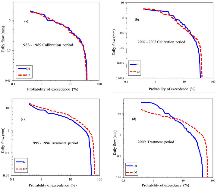
Figure 7. Flow duration curves of D1 and D2 during calibration (7(a) and 7(b)) and treatment (7(c) and 7(d)) periods. The main focus is shifts in the point of “cease to flow” (where the curves meet the abscissa axis) and differences in curve slopes during different periods.
cause the points of cease to flow (point where the curves meet the abscissa axis) are less than 70% probability of exceedence. Thus the two watersheds are under zeroflow conditions at least 30% of the respective calibration and treatment periods. The FDCs of D1 and D2 are similar during calibration period 1 (1988-1989) but slightly different during the low flows of calibration period 2 (2007-2008) after treatment reversal. For both treatment periods of harvesting, there are increased flows on D1 and D2 compared to calibration periods. This is demonstrated by higher flow magnitudes and a shift to the right of the respective points of cease to flow. The treatment effects of harvesting are demonstrated by higher flows on the treatment watershed (D2 for period 1 and D1 for period 2) for flows corresponding to probabilities of exceedence of less than 5%.
Comparison of FDCs during the two calibration periods shows a difference between slopes of the two periods. The slopes during calibration period 2 are steeper than slopes of calibration period 1. According to [68], steeper slopes are indicative of higher flow variability (also reflected by higher standard deviation in Table 2) with limited surface and subsurface storage. Although the low-flow characteristics for D1 and D2 are similar during calibration period 1, the low-flows of D2 are higher during calibration period 2. This slight increase in storage for D2 may be attributed to soil modifications during treatment period 1 and difference in surface depression storage. The difference in flow variability and storage explains the difference in D1 and D2 flow relationships during the two calibration periods (Figure 6(a)).
For both treatment periods, the point of cease to flow shifts from about 40% probability of exceedence to 50% for D1 and to 70% for D2 during the first treatment period and to 45% for D1 and 70% for D2 during the second treatment period. Therefore, after treatment period 1, D2 consistently had more low-flows based on point of cease to flow (more storage). During treatment period 1, treatment effects are evident throughout the entire FDC (during high and low flow regimes) because the FDC of D2 is consistently higher than FDC of D1. However, during treatment period 2, treatment effects are more pronounced for flows corresponding to probabilities of exceedence less than 5%.
4. Summary and Conclusions
The study explored the consistency and similarity of daily water table elevation and flow relationships between two adjacent paired watersheds (D1 and D2) before and after reversal of treatment on the two watersheds during a 21-year span. The studied treatment was the effect of operational silvicultural practices of harvesting, shearing, and bedding on daily water table elevation (WTE) and daily flow of artificially drained pine forested coastal watersheds. Before the treatment reversal (calibration period: 1988-1989, treatment period: 1995-1996), D1 was under control while D2 was under treatment and vice-versa after reversal of treatment (calibration period: 2007-2008, treatment period: 2009). Thus, this unique data provided an opportunity to test a key assumption of the paired watershed study design, which is consistency of relationship between hydrological responses of the paired watersheds over time, as a surrogate for replicated design. Preliminary analysis using cumulative sums of squared recursive residuals test showed no significant structural shifts in daily WTE and daily flow data during the two calibration and treatment periods. A simple linear equation was fitted for the daily WTE and daily flow relationships. The regression coefficients were estimated by bootstrapped geometric mean regression to minimize effects of data autocorrelation and the drawbacks of using ordinary least squares regression analysis. Cumulative treatment effects for daily WTE and daily flow were estimated six months after treatment for the two treatment periods.
Water table elevation calibration relationships before and after the treatment reversals were similar with no significant statistical difference (α = 0.05). However, the WTE relationships during the two treatment periods were significantly different. The cumulative treatment effects on WTE after the treatment reversal were 138% greater than cumulative treatment effects before the reversal (18.9 cm/day vs. 45 cm/day). Both the calibration and treatment daily flow relationships before and after treatment reversal were not similar. There was a 33.3% increase in treatment effect on flow after treatment reversal compared to before (0.60 mm/day vs. 0.80 mm/day). The difference in WTE and flow response to treatment reversal was attributed to modifications of soil properties of the top soil layer (0 - 70 cm) such that 12 years after treatment on D2 (from 1995 when D2 was under treatment to 2007 when D2 was under control), the WTE had returned to 1988 baseline levels while flow response had not.
The results show that even for two adjacent similar small watersheds (drainage area less than 30 ha or 0.3 km2), the choice of the control and treatment watersheds in addition to the season in which harvesting is implemented, influence the cumulative treatment effects on WTE and flow. Since the WTE calibration relationships were similar, the authors believe, the paired watershed approach under-estimated treatment effects when D2 was clear-cut (because mean [WTE2-WTE1] < 0 during calibration period) and over-estimated treatment effects when D1 was clear-cut (mean [WTE1-WTE2] > 0 during calibration period). Age difference of 20 years (11 - 12 years versus 34 - 35 years), between pine stands on control and treatment watersheds during 2007 to 2008 calibration gave the same WTE relationship as age difference of zero (both watersheds under 14 - 15 years old pine stands) during 1988 to 1989 calibration period.
REFERENCES
- K. J. McGuire and G. E. Likens, “Historical Roots of Forest Hydrology and Biogeochemistry,” Forest Hydrology and Biogeochemistry, Vol. 216, 2011, pp. 3-26. doi:10.1007/978-94-007-1363-5_1
- V. Andréassian, “Waters and Forests: From Historical Controversy to Scientific Debate,” Journal of Hydrology, Vol. 291, No. 1-2, 2004, pp. 1-27. doi:10.1016/j.jhydrol.2003.12.015
- R. L. Beschta, “Long-Term Patterns of Sediment Production Following Road Construction and Logging in the Oregon Coast Range,” Water Resources Research, Vol. 14, No. 6, 1978, pp. 1011-1016. doi:10.1029/WR014i006p01011
- T. A. Burton, “Effects of Basin-Scale Timber Harvest on Water Yield and Peak Streamflow,” Journal of the American Water Resources Association, Vol. 33, No. 6, 1997, pp. 1187-1196. doi:10.1111/j.1752-1688.1997.tb03545.x
- K. Cromack Jr., F. Swanson and C. Grier, “A Comparison of Harvesting Methods and Their Impact on Soils and Environment in the Pacific Northwest,” Proceedings of 5th North American Forest Soils Conference, Colorado State University Press, Fort Collins, 6-9 August 1978, pp. 449-476.
- J. D. Hewlett, H. Pos and D. Doss, “Effect of Clear-Cut Silviculture on Dissolved Ion Export,” Water Resources Research, Vol. 20, No. 7, 1984, pp. 1030-1038. doi:10.1029/WR020i007p01030
- J. D. Hewlett and L. Pienaar, “Design and Analysis of the Catchment Experiment,” 1973.
- J. W. Hornbeck, C. Martin, R. Pierce, F. Bormann, G. Likens and J. Eaton, “Clearcutting Northern Hardwoods: Effects on Hydrologic and Nutrient Ion Budgets,” Forest Science, Vol. 32, No. 3, 1986, pp. 667-686.
- C. W. Martin and R. S. Pierce, “Clearcutting Patterns Affect Nitrate and Calcium in Streams of New Hampshire,” Journal of Forestry, Vol. 78, No. 5, 1980, pp. 268-272.
- H. Riekerk, “Influence of Silvicultural Practices on the Hydrology,” Water Resources Research, Vol. 25, No. 4, 1989, pp. 713-719. doi:10.1029/WR025i004p00713
- W. T. Swank and J. D. Helvey, “Reduction of Streamflow Increases Following Regrowth of Clearcut Hardwood Forests,” 1970, pp. 346-360.
- J. C. Clausen and J. Spooner, “Paired Watershed Study Design,” Office of Wetlands, Oceans and Watersheds, Environmental Protection Agency, Washington DC, 1993.
- W. E. Jokela and M. D. Casler, “Transport of Phosphorus and Nitrogen in Surface Runoff in a Corn Silage System: Paired Watershed Methodology and Calibration Period Results,” 2011.
- K. King, P. Smiley Jr., B. Baker and N. Fausey, “Validation of Paired Watersheds for Assessing Conservation Practices in the Upper Big Walnut Creek Watershed, Ohio,” Journal of Soil and Water Conservation, Vol. 63, No. 6, 2008, pp. 380-395.
- A. Lemke, J. Herkert, T. Lindenbaum, M. Herbert, K. Kirkham, T. Tear, et al., “Evaluating Agricultural Best Management Practices in Tile-Drained Subwatersheds of the Mackinaw River, Illinois,” Journal of Environmental Quality, Vol. 40, 2011, pp. 1215-1228.
- R. Kallenbach, H. E. Garrett and R. P. Udawatta, “Agroforestry Buffers for Nonpoint Source Pollution Reductions from Agricultural Watersheds,” Journal of Environmental Quality, Vol. 40, No. 4, 2011, pp. 800-806.
- B. R. Paudel, R. P. Udawatta and S. H. Anderson, “Agroforestry and Grass Buffer Effects on Soil Quality Parameters for Grazed Pasture and Row-Crop Systems,” Applied Soil Ecology, Vol. 48, No. 2, 2011, pp. 125-132. doi:10.1016/j.apsoil.2011.04.004
- R. P. Udawatta, R. J. Kremer, H. E. Garrett and S. H. Anderson, “Soil Enzyme Activities and Physical Properties in a Watershed Managed under Agroforestry and Row-Crop Systems,” Agriculture, Ecosystems & Environment, Vol. 131, No. 1-2, 2009, pp. 98-104. doi:10.1016/j.agee.2008.06.001
- R. P. Udawatta, J. J. Henderson, G. S. Garrett and E. Harold, “Agroforestry Practices, Runoff, and Nutrient Loss,” Journal of Environmental Quality, Vol. 31, No. 4, 2002, p. 1214.
- K. S. Veum, K. W. Goyne, P. P. Motavalli and R. P. Udawatta, “Runoff and Dissolved Organic Carbon Loss from a Paired-Watershed Study of Three Adjacent Agricultural Watersheds,” Agriculture, Ecosystems & Environment, Vol. 130, No. 3-4, 2009, pp. 115-122. doi:10.1016/j.agee.2008.12.006
- P. L. Bishop, W. D. Hively, J. R. Stedinger, M. R. Rafferty, J. L. Lojpersberger and J. A. Bloomfield, “Multivariate Analysis of Paired Watershed Data to Evaluate Agricultural Best Management Practice Effects on Stream Water Phosphorus,” Journal of Environmental Quality, Vol. 34, No. 3, 2005, pp. 1087-1101.
- D. B. Jaynes, D. Dinnes, D. Meek, D. Karlen, C. Cambardella and T. Colvin, “Using the Late Spring Nitrate Test to Reduce Nitrate Loss within a Watershed,” 2004.
- K. E. Schilling, “Chemical Transport from Paired Agricultural and Restored Prairie Watersheds,” Journal of Environmental Quality, Vol. 31, No. 4, 2002, pp. 1184- 1193.
- D. M. Amatya, J. Gilliam, R. Skaggs, M. Lebo and R. Campbell, “Effects of Controlled Drainage on Forest Water Quality,” Journal of Environmental Quality, Vol. 27, No. 4, 1998, pp. 923-935 doi:10.2134/jeq1998.00472425002700040029x
- D. M. Amatya, J. D. Gregory and R. Skaggs, “Effects of Controlled Drainage on Storm Event Hydrology in a Loblolly Pine Plantation,” Journal of the American Water Resources Association, Vol. 36, No. 1, 2000, pp. 175-190. doi:10.1111/j.1752-1688.2000.tb04258.x
- D. M. Amatya, R. Skaggs and J. Gregory, “Effects of Controlled Drainage on the Hydrology of Drained Pine Plantations in the North Carolina Coastal Plain,” Journal of Hydrology, Vol. 181, No. 1-4, 1996, pp. 211-232. doi:10.1016/0022-1694(95)02905-2
- J. Shanley and B. Wemple, “Effects of Mountain Resort Development—A Case Study in Vermont USA,” 2012.
- J. C. Loftis, L. H. MacDonald, S. Streett, H. K. Iyer and K. Bunte, “Detecting Cumulative Watershed Effects: The Statistical Power of Pairing,” Journal of Hydrology, Vol. 251, No. 1-2, 2001, pp. 49-64. doi:10.1016/S0022-1694(01)00431-0
- L. S. Prokopy, Z. Asligül Göçmen, J. Gao, S. B. Allred, J. E. Bonnell, K. Genskow, et al., “Incorporating Social Context Variables Into Paired Watershed Designs to Test Nonpoint Source Program Effectiveness1,” Journal of the American Water Resources Association, Vol. 47, No. 1, 2011, pp. 196-202.
- E. Mellina and S. G. Hinch, “Overview of Large-Scale Ecological Experimental Designs and Recommendations for the British Columbia Watershed Restoration Program,” Ministry of Environment, Lands and Parks and Ministry of Forestry, Vancouver, 1995.
- A. L. Vogl and V. L. Lopes, “Evaluating Watershed Experiments through Recursive Residual Analysis,” Journal of Irrigation and Drainage Engineering, Vol. 136, No. 5, 2010, pp. 348-353. doi:10.1061/(ASCE)IR.1943-4774.0000203
- Y. Alila, P. Kuras, M. Schnorbus and R. Hudson, “Forests and Floods: A New Paradigm Sheds Light on AgeOld Controversies,” Water Resources Research, Vol. 45, No. 8, 2009, Article ID: W08416. doi:10.1029/2008WR007207
- P. K. Kuraś, Y. Alila and M. Weiler, “Forest Harvesting Effects on the Magnitude and Frequency of Peak Flows Can Increase with Return Period,” Water Resources Research, Vol. 48, No. 1, 2012, Article ID: W01544. doi:10.1029/2011WR010705
- N. A. Som, N. P. Zégre, L. M. Ganio and A. E. Skaugset, “Corrected Prediction Intervals for Change Detection in Paired Watershed Studies,” Hydrological Sciences Journal, Vol. 57, No. 1, 2012, pp. 134-143. doi:10.1080/02626667.2011.637494
- J. L. Boggs and G. Sun, “Urbanization Alters Watershed Hydrology in the Piedmont of North Carolina,” Ecohydrology, Vol. 4, No. 2, 2011, pp. 256-264.
- J. C. Bathurst, “Predicting Impacts of Land Use and Climate Change on Erosion and Sediment Yield in River Basins Using SHETRAN,” Handbook of Erosion Modelling, 2011, pp. 263-288.
- Z. Liu, S. Tong, C. Jeganathan, P. Roy, M. Jha, Z. Yang, et al., “Using HSPF to Model the Hydrologic and Water Quality Impacts of Riparian Land-Use Change in a Small Watershed,” Journal of Environmental Informatics, Vol. 17, No. 1, 2011, pp. 1-14. doi:10.3808/jei.201100182
- S. Tian, M. A. Youssef, R. W. Skaggs, D. M. Amatya, and G. Chescheir, “DRAINMOD-FOREST: Integrated Modeling of Hydrology, Soil Carbon and Nitrogen Dynamics, and Plant Growth for Drained Forests,” Journal of Environmental Quality, Vol. 41, No. 3, 2012, pp. 764- 782.
- M. Wiley, D. Hyndman, B. Pijanowski, A. Kendall, C. Riseng, E. Rutherford, et al., “A Multi-Modeling Approach to Evaluating Climate and Land Use Change Impacts in a Great Lakes River Basin,” Hydrobiologia, Vol. 657, No. 1, 2010, pp. 243-262. doi:10.1007/s10750-010-0239-2
- W. H. McDowell, “Comparative Watershed Studies-Opportunities and Limitations,” ILTER Regional Workshop, Budapest, 2000.
- P. Schleppi, “Forested Water Catchments in a Changing Environment,” Forest Management and the Water Cycle, Vol. 212, 2011, pp. 89-110.
- C. R. Ford, S. H. Laseter, W. T. Swank and J. M. Vose, “Can Forest Management Be Used to Sustain Water- -Based Ecosystem Services in the Face of Climate Change?” Ecological Applications, Vol. 21, 2011, pp. 2049-2067.
- D. M. Amatya, R. Skaggs and J. Gilliam, “Hydrology and Water Quality of a Drained Loblolly Pine Plantation in Coastal North Carolina,” American Society of Agricultural and Biological Engineers, St. Joseph, 2006.
- J. W. Hornbeck, M. Adams, E. Corbett, E. Verry and J. Lynch, “Long-Term Impacts of Forest Treatments on Water Yield: A Summary for Northeastern USA,” Journal of Hydrology, Vol. 150, No. 2-4, 1993, pp. 323-344. doi:10.1016/0022-1694(93)90115-P
- J. W. Hornbeck, C. Martin and C. Eagar, “Summary of Water Yield Experiments at Hubbard Brook Experimental Forest, New Hampshire,” Canadian Journal of Forest Research, Vol. 27, No. 12, 1997, pp. 2043-2052.
- E. McCarthy, R. Skaggs, and P. Farnum, “Experimental Determination of the Hydrologic Components of a Drained Forest Watershed,” Transactions of the ASAE, Vol. 34, No. 5, 1991, pp. 2031-2039.
- D. M. Amatya and R. Skaggs, “Long-Term Hydrology and Water Quality of a Drained Pine Plantation in North Carolina,” Transactions of the ASAE, Vol. 54, No. 6, 2011, pp. 2087-2098.
- E. F. Brater and H. W. King, “Handbook of Hydraulics: for the Solution of Hydraulic Engineering Problems,” McGraw-Hill, New York, 1996.
- D. M. Amatya, R. Skaggs, C. Blanton and J. Gilliam, “Hydrologic and Water Quality Effects of Harvesting and Regeneration of a Drained Pine Forest,” American Society of Agricultural and Biological Engineers, St. Joseph, 2006.
- R. L. Brown, J. Durbin and J. M. Evans, “Techniques for Testing the Constancy of Regression Relationships over Time,” Journal of the Royal Statistical Society. Series B (Methodological), Vol. 37, No. 2, 1975, pp. 149-192.
- J. S. Galpin and D. M. Hawkins, “The Use of Recursive Residuals in Checking Model Fit in Linear Regression,” The American Statistician, Vol. 38, No. 2, 1984, pp. 94- 105.
- J. P. LeSage and R. K. Pace, “Introduction to Spatial Econometrics,” Chapman & Hall/CRC, London, 2009. doi:10.1201/9781420064254
- R. E. Plotnick, “Application of Bootstrap Methods to Reduced Major Axis Line Fitting,” Systematic Biology, Vol. 38, No. 2, 1989, pp. 144-153. doi:10.1093/sysbio/38.2.144
- W. Ricker, “Linear Regressions in Fishery Research,” Journal of the Fisheries Board of Canada, Vol. 30, No. 3, 1973, pp. 409-434. doi:10.1139/f73-072
- B. McArdle, “The Structural Relationship: Regression in Biology,” Canadian Journal of Zoology, Vol. 66, No. 11, 1988, pp. 2329-2339. doi:10.1139/z88-348
- C. Cunnane, “Unbiased Plotting Positions—A Review,” Journal of Hydrology, Vol. 37, No. 3-4, 1978, pp. 205- 222. doi:10.1016/0022-1694(78)90017-3
- V. Baldwin, “Green and Dry-Weight Equations for Above-Ground Components of Planted Loblolly Pine Trees in the West Gulf Region,” Southern Journal of Applied Forestry, Vol. 11, No. 4, 1987, pp. 212-218.
- C. Blanton, R. Skaggs, D. Amatya and G. Chescheir, “Soil Hydraulic Property Variations during Harvest and Regeneration of Drained, Coastal Pine Plantations,” 1998, pp. 12-16.
- J. M. Grace, R. W. Skaggs and D. K. Cassel, “Soil Physical Changes Associated with Forest Harvesting Operations on an Organic Soil,” Soil Science Society of America Journal, Vol. 70, No. 2, 2006, pp. 503-509. doi:10.2136/sssaj2005.0154
- [61] R. W. Skaggs, D. M. Amatya, G. M. Chescheir, C. D. Blanton and J. W. Gilliam, “Effects of Drainage and Management Practices on Hydrology of Pine Plantation,” Hydrology and Management of Forested Wetlands, St. Joseph, 2006.
- [62] Y. J. Xu, J. A. Burger, W. M. Aust, S. C. Patterson, M. Miwa and D. P. Preston, “Changes in Surface Water Table Depth and Soil Physical Properties after Harvest and Establishment of Loblolly Pine (Pinus taeda L.) in Atlantic Coastal Plain Wetlands of South Carolina,” Soil and Tillage Research, Vol. 63, No. 3-4, 2002, pp. 109-121. doi:10.1016/S0167-1987(01)00226-4
- [63] M. A. Rab, “Recovery of Soil Physical Properties from Compaction and Soil Profile Disturbance Caused by Logging of Native Forest in Victorian Central Highlands, Australia,” Forest Ecology and Management, Vol. 191, No. 1-3, 2004, pp. 329-340. doi:10.1016/j.foreco.2003.12.010
- [64] M. H. Eisenbies, J. A. Burger, W. M. Aust and S. C. Patterson, “Loblolly Pine Response to Wet-Weather Harvesting on Wet Flats after 5 Years,” Water, Air, & Soil Pollution: Focus, Vol. 4, No. 1, 2004, pp. 217-233. doi:10.1023/B:WAFO.0000012817.20157.d3
- [65] M. Miwa, W. M. Aust, J. A. Burger, S. C. Patterson and E. A. Carter, “Wet-Weather Timber Harvesting and Site Preparation Effects on Coastal Plain Sites: A Review,” Southern Journal of Applied Forestry, Vol. 28, No. 3, 2004, pp. 137-151.
- [66] G. Sun, S. G. McNulty, J. P. Shepard, D. M. Amatya, H. Riekerk, N. B. Comerford, et al., “Effects of Timber Management on the Hydrology of Wetland Forests in the Southern United States,” Forest Ecology and Management, Vol. 143, No. 1-3, 2001, pp. 227-236. doi:10.1016/S0378-1127(00)00520-X
- [67] G. Sun, H. Riekerk and L. V. Kornhak, “Ground-WaterTable Rise after Forest Harvesting on Cypress-Pine Flatwoods in Florida,” Wetlands, Vol. 20, No. 1, 2000, pp. 101-112. doi:10.1672/0277-5212(2000)020[0101:GWTRAF]2.0.CO;2
- [68] C. Bliss and N. Comerford, “Forest Harvesting Influence on Water Table Dynamics in a Florida Flatwoods Landscape,” Soil Science Society of America Journal, Vol. 66, No. 4, 2002, pp. 1344-1349. doi:10.2136/sssaj2002.1344
- [69] J. K. Searcy, “Flow-Duration Curves Manual of Hydrology: Part 2. Low-Flow Techniques,” US Department of Interior, Washington, 1959.