Open Journal of Fluid Dynamics
Vol.4 No.1(2014), Article ID:44088,20 pages DOI:10.4236/ojfd.2014.41007
The Influence of Boundaries on the Stability of Compositional Plumes
Khaled S. Al-Mashrafi, Ibrahim A. Eltayeb
Department of Mathematics and Statistics, College of Science, Sultan Qaboos University, Muscat, Oman
Email: P001175@student.squ.edu.om
Copyright © 2014 by authors and Scientific Research Publishing Inc.
This work is licensed under the Creative Commons Attribution International License (CC BY).
http://creativecommons.org/licenses/by/4.0/


Received 13 February 2014; revised 13 March 2014; accepted 20 March 2014
ABSTRACT
The influence of boundaries on the dynamics of a compositional plume is studied using a simple model in which a column of buoyant fluid rises in a less buoyant fluid bounded by two vertical walls with a finite distance apart. The problem is governed by four dimensionless parameters: The Grashoff number, R, which is a measure of the difference in concentration of light material of the plume to its surrounding fluid, the Prandtl number, σ, which is the ratio of viscosity, ν, to thermal diffusivity, κ, the thickness of the plume, 2x0, and the distance, d, between the two vertical walls relative to the salt-finger length scale. The influence of the boundary on the fluxes of material, heat, and buoyancy is examined to find that the buoyancy flux possesses a local maximum for moderate to small thicknesses of the plume when they lie close to the wall. This has the effect of introducing a region of instability for thin plumes near the wall with an asymptotically larger growth rate. In addition, the presence of the boundary suppresses the three-dimensional instabilities present in the unbounded domain and allows only two-dimensional instabilities for moderate to small distances between the bounding walls.
Keywords:Compositional Plumes; Flux; Stability; Growth Rate; Bounded Domain

1. Introduction
Studies on the dynamics of fluid alloys are relevant to industrial (e.g., Rees and Worster [1] and references therein), environmental (e.g., Wells et al. [2] and references therein) and geophysical (e.g., Loper [3] , Moffatt [4] , Al-Lawatiaet al. [5] ), applications. Consequently, there has been considerable interest in studying the various aspects of the dynamics of fluid alloys.
In industrial applications, one of the problems the iron casting industry faces is the appearance of freckles in iron bars causing their weakness. When iron ore is poured into molds or designs, air trapped at the bottom of the design rises in the form of thin filaments into the liquid iron. When the iron solidifies, these filaments form trapped air pockets that appear as very thin black strips along the outer surface of the iron bar and lead to a weakness in the iron bar. The experimental work of Copley et al. [6] showed the appearance of plumes rising as thin filaments from a mushy layer. This work was extended by a number of authors (see, e.g. Huppert [7] , Chen and Chen [8] , Tait and Jaupart [9] , Jellinek et al. [10] , Classen et al. [11] , Aussillous et al. [12] , Pol et al. [13] ). It has been observed that the behaviour of plumes emanating from mushy layers depends on whether they are near the walls of the container or not (see, e.g., Hellawell et al. [14] ).
Theoretical studies of a compositional plume rising in a fluid of infinite extent have shown that the plume is unstable (see, e.g., Eltayeb and Loper [15] ) even for small Grashoff numbers. Moreover, this is found to be true even if the plume is subject to rotation or in the presence of a magnetic field even if another plume is also present [5] [16] -[18] .
The main purpose of this study is to examine the influence of boundaries on the dynamics of compositional plumes. For this purpose, we introduce boundaries to the model discussed by Eltayeb and Loper [16] . This is a simple model that neglects material diffusion, which is known to be small, compared to viscous and thermal diffusion [15] . A finite column of compositionally buoyant fluid contained between two vertical interfaces, referred to as a Cartesian plume, is rising in a fluid bounded by two parallel walls enclosing the plume (see figure 1). The neglect of material diffusion allows us to adopt a function of concentration of light material that is simple with the consequence that an analytical solution is obtained. This allows us to examine the dynamics of the plume in a bounded region in the whole parameter space and thus get some insight into the influence of the boundaries on the dynamics of a plume.
In section 2, we formulate the problem, which involves four dimensionless parameters: the Grashoff number,  , which measures the ratio of the buoyancy force to the viscous force, the Prandtl number,
  , which measures the ratio of viscosity force to the thermal diffusivity, defined by
 (1)
(1)
where  and
and  are characteristic velocity and length-scale, respectively (see equations (9) and (10) below), and
  and
and  are kinematic viscosity and thermal diffusivity, respectively, and the thickness of the plume,
  , and the distance between the two bounding walls,
  , made dimensionless using the length scale
 .
.
In section 3, we use a top-hat profile of the concentration of light material to obtain a solution representing a plume of thickness , rising between two rigid sidewalls a distance,
  , apart. We discuss the influence of the presence of the sidewalls on the basic state flow and temperature as well as the associated fluxes of material, heat, and buoyancy. It is found that the presence of the boundaries increases the amplitude of the basic state vertical velocity of the plume flow. The fluxes of material, heat and buoyancy are presented as contours in the
  plane, where
  is a measure of the distance between plume and the nearest sidewall.
In section 4, we examine the stability of the plume. This poses an eigenvalue problem for the growth rate  of the perturbations. In the absence of the walls, the plume is always unstable for small values of the Grashoff number,
  , and the instability takes the form of one of two uncoupled modes, depending on the values of the dimensionless parameters: a varicose (V) mode, in which the two interfaces of the plume are out-of-phase or a sinuous (S) mode, in which case the two interfaces are in-phase. When the walls are introduced, the same two modes persist but are modified by the presence of the walls. We refer to them below as the modified varicose (MV) and modified sinuous (MS) modes. The stability results are discussed in section 5. In particular, it will be shown that the influence of the sidewalls is quite complicated. While it tends to stabilise the plume if it is equidistant from the two sidewalls, it can destabilise the plume if it is nearer to one sidewall than to the other. Some concluding remarks are made in section 6.
2. Formulation of the Problem
We consider a two-component incompressible fluid in which the concentration of the solvent component (light material) is  and the temperature is
 . The two fluids have the same kinematic viscosity,
  , and thermal diffusivity,
 . The system is governed by the equations of motion, mass, heat, concentration of the light material, and state. These equations are
 (2)
(2)
 (3)
(3)
 (4)
(4)
 (5)
(5)
 (6)
(6)
where  is the velocity vector,
  the pressure, g the uniform acceleration of gravity,
  is the upward unit vector, t the time,
  the coefficient of thermal expansion,
  the coefficient of compositional expansion,
  the density,
  reference values, and we have assumed that the fluid is Boussinesq. The Equations (2)-(6) allow a hydrostatic balance governed by
 (7)
(7)
Motivated by the experimental work on plumes rising from mushy layers, we take a temperature profile
 (8)
(8)
where  is a positive constant and
  is the vertical coordinate measured vertically upwards, so that the temperature increases with height making the fluid stably stratified thermally and any instabilities will be due to transport of material.
We now cast the equations - into dimensionless form. It is found that in order to maintain the effects of temperature variations and compositional variations, we use the salt-finger length scale defined by
 (9)
(9)
and a velocity unit with the definition
 , (10)
so that the ensuing motions are driven by the plume flow transporting the light material,  , upwards. Here
  is the maximum amplitude of the concentration of light material. We further choose
 ,
,  and
and
 as units of temperature, time and pressure, respectively, and express the equations in dimensionless form as
 (11)
(11)
 (12)
(12)
 (13)
(13)
 (14)
(14)
Here the dimensionless parameters  and
and  are the Grashoff and Prandtl numbers defined in equation (1) above.
We define a Cartesian coordinate system  in which
  is vertically upwards and
 ,
,  are horizontal with the
  -axis normal to the bounding walls (see figure 1). A column of fluid of finite thickness,
  , rising vertically upwards in a fluid of different concentration and bounded on either side by vertical walls,
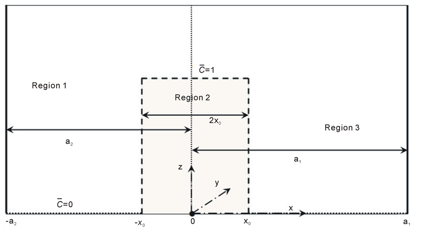
Figure 1. The geometry of the problem showing the profile of the basic state concentration of light material representing a plume of width,  , and concentration, 1, rising vertically in a fluid of width,
  , and concentration, 0. Two vertical planes bound the plume on either side such that the center of the plume is a distance
  from the wall on the right and
  from the wall on the left.
a distance  apart. We choose the origin such that the plume interfaces are situated at
  and the walls at
  and
and . The region is unbounded in the
  and
and  directions. In comparison with the plumes observed in experiments on mushy layers (see, e.g., Huppert [7] ), our model is different in that it is unbounded in the
  and
and  directions. We feel that both assumptions can be adopted for the following reasons: First, the studies in [16] [17] showed good agreement between the stability results of the circular cylindrical plume and the Cartesian plume. Secondly, experimental work on mushy layers and the formation of plumes shows that fully developed plumes rise to heights 200 times their thickness [14] , and we can approximate the situation for a fully developed plume by considering it infinite in the vertical direction.
We can now take the flow variables to have the form
 (15)
(15)
 (16)
(16)
 (17)
(17)
 (18)
(18)
such that the variables with subscript  represent hydrostatic balance and given (in dimensionless form) by
 (19)
(19)
 (20)
(20)
The variables with an “overbar” are basic state variables dependent only on the horizontal coordinate , because the horizontal variations of the vertical plume flow caused by the difference in composition between the plume and the surrounding fluid imposes a horizontal variation of temperature.The variables with a “dagger” indicate a perturbation of small amplitude
 .
.
Substituting the expressions (15)-(18) into the system (11) - (14), the terms independent of  give the basic state equations, which depend on
  only
only
 (21)
(21)
 (22)
(22)
These equations are discussed in section 3 below.
The order  terms in the equations provide the linearised perturbation equations as follows


 (23)
(23)
 (24)
(24)
 (25)
(25)
 (26)
(26)
The perturbation equations are solved in section 4 below.
3. The Basic State
Equation (14) is automatically satisfied for the basic state and we are free to choose a concentration function . Since we are extending the study by Eltayeb and Loper [16] , we will adopt their choice of
 . Thus
 (27)
(27)
Consider the basic state equations (21) and (22). Define
 (28)
(28)
Then
 (29)
(29)
The equation (29) is subject to the boundary conditions
 (30)
(30)
The solution is
 (31)
(31)
where  and
and  are defined by
 (32)
(32)
A sample of the profiles of the solutions  and
and  is plotted for different values of the plume thickness
 , the distance
  and
and  in figure 2. The profiles are symmetric when the plume is situated half-way between the sidewalls. The oscillatory nature of the velocity profile introduces negative flow
Figure 2. The profiles of the basic state velocity,  , and temperature,
  , for different values of plume thickness,
  , and distance,
  , from the wall on the left when
 . (a) and (c) refer to
  and
and , respectively, when the plume is positioned half-way between the two sidewalls and the labels i, ii, iii correspond to
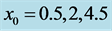 , respectively. (b) and (d) refer to
  and
and  when
when  and the labels iv, v, vi correspond to
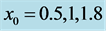 , respectively. Note that when the plume is wide, the flow is oscillatory within the plume and it slows down in the middle of the plume, while the flow of the plume is enhanced in the center of the plume when the plume approaches the wall.
(i.e., downwards flow) within the plume when it is wide, and this has an effect on the net transport of material by the plume. The wide plume is also associated with a temperature profile that is almost uniform in the main body of the plume. If the position of the plume moves towards a sidewall, symmetry is broken. Here the downward flow outside the plume is partially suppressed in the narrow region between the plume and the nearest wall and strengthened on the far side. Such behavior will lead to the modification of the modes of instability in the absence of the sidewalls.
The basic state solution is associated with fluxes of heat,  , material,
  , and buoyancy,
  , which are non-dimensionalised using the units
 ,
,  and
and respectively. They are given by
 (33)
(33)
(cf. [15]). The integration is straightforward and leads to
 (34)
(34)
 (35)
(35)
where ,
,  and
and  are given by
 (36)
(36)
 (37)
(37)
 (38)
(38)
The fluxes are presented in the  plane in figure 3. The presence of the sidewalls has complicated the behavior of the fluxes as compared to the case of infinite surrounding fluid. For a fixed position of the plume (i.e., fixed
 ) relative to the wall, gradual increase in the thickness of the plume is associated with an increase in the downward heat flux. For plumes of thickness less than about 2, the heat flux is almost a constant as the plume moves towards a sidewall. For plumes with larger thickness, the heat flux increases as the wall is approached. The upward material flux behaves similarly if the distance from the wall is less than about 4.5. For larger distances from the sidewalls, the material flux increases as
  increases from zero reaching a maximum before it decreases to a minimum and starts to increase again to a larger value as
  approaches
  and the plume interface approaches a sidewall. The buoyancy flux, which is the net system flux, possesses two local maxima and a minimum. The local maximum with the largest value is situated on the boundary at
 , while the other one is situated half-way between the two sidewalls and about the same value of
 . The minimum occurs for
  and lies half-way between the sidewalls. The buoyancy flux per unit area, illustrated in (d), has the same general behavior as the buoyancy flux but the positions of the two local maxima and minimum are different.
4. Solution of the Eigenvalue Problem
In this section, we solve the eigenvalue problem posed by the perturbation equations (23)-(26) and the relevant boundary conditions to obtain expressions for the growth rate. Our interest lies in the instability produced by the buoyant fluid in the plume. We assume that the interface at the plane  is given a small harmonic disturbance of the form
 (39)
(39)
where  and
and  are the horizontal and vertical wavenumbers,
  refers to the complex conjugate, and
  is a complex constant, which can be expressed as
 (40)
(40)
 and
and  will be referred to as the real and imaginary parts of
 . The stability of the plume is determined by the sign of
 . If it is negative for all possible values of the wavenumbers
  and
and , then the plume is stable, but the system is rendered unstable if any pair
  of wavenumbers gives a positive value of
 . If the preferred mode occurs for
 ,
,  both non-zero, it is referred to as a 3-dimensional mode but if any one of them vanishes it is 2-dimensional. If the maximum value of
  vanishes, the plume is neutrally stable.
The disturbance (39) will propagate into the system, and affect the second interface and the variables of the system to produce the perturbations. The disturbance at the interface  can be written in the form
 (41)
(41)
where  is the amplitude of the displacement of the interface at
 , and will be determined by the solution.
The perturbation variables produced by the disturbance (39) can be expressed in the form
 (42)
(42)
where the factors ,
,  and
and  are introduced in the variables
 ,
,  and
and , respectively, for convenience.
Substituting the variables (42) into (23)-(26), we obtain the following ordinary differential equations in 
 (43)
(43)
 (44)
(44)
 (45)
(45)
 (46)
(46)
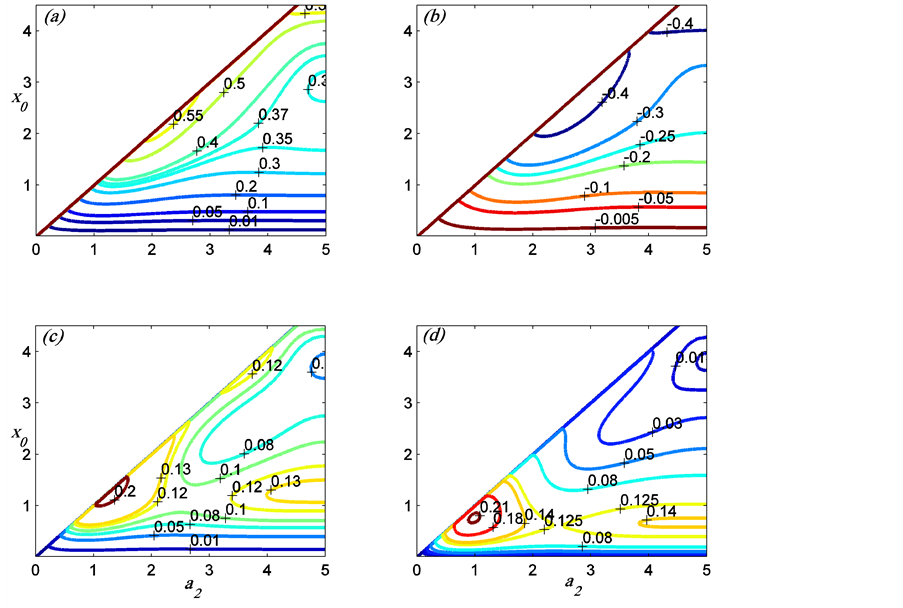
Figure 3. The contours of the basic state fluxes of the top-hat bounded plume in the  plane; (a) material flux,
  , (b) heat flux,
  , (c) buoyancy flux,
  and (d) buoyancy flux per unit area
  when
when . Note that the heat and material fluxes are larger at the sidewall, the buoyancy flux has a maximum value of 0.215, when
 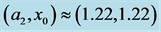 and the buoyancy flux per unit area has a maximum 0.212 at
 , and both maxima lie on the sidewall. The fluxes are shown for half the interval because they are symmetric about the middle plane between the sidewalls.
 (47)
(47)
 (48)
(48)
Here we have used
 (49)
(49)
The boundary conditions across the interfaces are (see, Eltayeb and Loper [16] )
 (50)
(50)
 (51)
(51)
 (52)
(52)
 (53)
(53)
In addition, the sidewalls are maintained at the hydrostatic temperature so that
 (54)
(54)
Equation (48) gives
 (55)
(55)
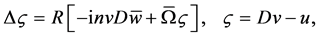
It was found that it is useful to derive the following three equations. First, differentiate (45) once and subtract (44) to get
 (56)
(56)
Where  is related to the vertical component of vorticity. Secondly, differentiate (43) once and subtract (44) to obtain
 . (57)
Thirdly, apply the operator  to (43) and use (44)-(46) to find
 (58)
(58)
The previous studies on a compositional plume showed that the plume flow is unstable for small value of Grashoff number [15] -[17] . This dimensionless number measures the strength of the plume, resulting from the maximum amplitude of the basic concentration. It transpires that instability is also present for small values of  here too. We then write
 (59)
(59)
where  indicates any of the perturbation variables
 ,
,  ,
,  ,
,  and
and .
.
Substituting the expressions (59) into the system (43)-(47), (56)-(58) and the associated boundary conditions (50)-(54), and equating the coefficients of  to zero, we get systems of ordinary differential equations which can be solved successively to find an expression for the growth rate. The two systems obtained for
  (referred to as Problem 0) and
  (referred to as problem 1) are sufficient to determine the stability of the interfaces, to leading order. It is found that the instability is present only in part of the parameter space, and it is necessary to consider the next order of the growth rate governed by Problem 1.
4.1. Problem 0
The coefficients of  in the system (45)-(47), (57)-(58) then consist of the equations
 (60)
(60)
 (61)
(61)
 (62)
(62)
 (63)
(63)
 , (64)
noting that (56) and the appropriate conditions imply that  everywhere. Taking note of (64), the boundary conditions can then be expressed as
 (65)
(65)
 (66)
(66)
 (67)
(67)
 (68)
(68)
We operate on equation (61) with , and use equations (62) and (63) to get
 (69)
(69)
The solution of the system (60)-(64) subject to the boundary conditions (65)-(67) is given by
 (70)
(70)
 (71)
(71)
where the superscript “i” in the solution refers to the region of the problem defined by
 (72)
(72)
(see figure 1) and  are the roots of the cubic equation
 (73)
(73)
with  given by
 (74)
(74)
The constants  and
and  for
for  are given by
 (75)
(75)
 (76)
(76)
 (77)
(77)
 (78)
(78)
 (79)
(79)
 (80)
(80)
with
 (81)
(81)
The application of the boundary conditions (68) gives an expression for the growth rate  and the displacement of the interface
 . This leads to
 (82)
(82)
 (83)
(83)
in which
 (84)
(84)
 (85)
(85)
 (86)
(86)
 (87)
(87)
Thus
 (88)
(88)
The properties of the roots of the cubic equation (73) render ,
,  real and hence the discriminant
  is real. It follows that
  is imaginary if
  and complex when
 . In the absence of the sidewalls, the two modes are such that the two interfaces of the plume are either in-phase giving a sinuous (S) solution or out-of-phase giving a varicose (V) solution. In both cases,
  is imaginary and the disturbances are neutral at this level of approximation of the growth rate. The introduction of the boundaries has destroyed the symmetry unless the plumes are situated halfway between the sidewalls.
It is informative to establish the relationship between the modes of the bounded plume defined by (88) and those of the unbounded one particularly that we expect the modes of the bounded plume to reduce to sinuous and varicose when the plume is positioned half-way between the two sidewalls. We take the limit , and find that
 (89)
(89)
 (90)
(90)
 (91)
(91)
and
 (92)
(92)
where  is defined by
 (93)
(93)
Substituting these expressions into the equation (88) for , we get
 (94)
(94)
The growth rate (94) is the same as the growth rate of the Cartesian plume obtained in Eltayeb and Loper [16] and the values of the displacement  shows that the phase of the interface at
  is either out-of-phase (varicose mode) with
  or in-phase (sinuous mode) with
 . It thus follows that the upper sign in (88) refers to a modification of the varicose mode, which we shall refer to as the modified varicose mode (MV) while the other will be denoted by the modified sinuous (MS) mode. The growth rate will be denoted by
 , where
  for the modified varicose and sinuous modes, respectively.
4.2. Problem 1
The coefficients of  in the perturbation equations (44)-(47), (56)-(58) give the set
 (95)
(95)
 (96)
(96)
 (97)
(97)
 (98)
(98)
 (99)
(99)
 (100)
(100)
 (101)
(101)
in which
 (102)
(102)
The associated boundary conditions are
 (103)
(103)
 (104)
(104)
 . (105)
The equations and boundary conditions (95)-(105) are solved in the Appendix A. They lead to the growth rate  given by
 (106)
(106)
where  is given by
 (107)
(107)
and  takes the symbols
  or
or . The expressions
 ,
,  ,
,  ,
,  and
and  are given by
 (108)
(108)
 (109)
(109)
 (110)
(110)
 (111)
(111)
 (112)
(112)
in which ,
,  ,
,  ,
,  ,
, and
and  are given in the Appendix.
It is noteworthy that because of the properties of the cubic equation (73) for , the zeroth order variables are all real. For wavenumbers for which the zeroth order solution is neutrally stable,
  is purely imaginary and the non-homogeneity of the equations of problem 1 are all imaginary. It then follows that the variables with subscript 1 are all imaginary. When we employ this result into the expression for
 , we find that
  is real, and consequently it will determine the stability of the plume outside the unstable regions of the zeroth order.
5. Discussions of the Results
The growth rates given by the expressions (88) and (106) were computed in the parameter space . For a given set of the parameters
 , the growth rate is maximized over
  and
and .
.
The maximum value,  , of
, of  and the corresponding wavenumbers
  and the vertical wave speed
  define the preferred mode of instability for that set of parameters.
First we consider equation (88). This growth rate at this level of approximation is independent of . As we mentioned previously, the stability of the plume at the leading order of approximation depends on
 . In figure 4 we show the isolines of
  in the wavenumber plane for some representative values of
  and
and . It is found that
  is negative for small values of
  and
and  indicating that instability at zeroth order is possible only if the plume is very thin and is close to the wall. Indeed, the maximisation of the growth rate (88) when
  shows that instability is possible only for values of
  not exceeding 0.25 and the unstable modes are two-dimensional and propagate vertically upwards (figure 5). In the calculations, the discrimnant and the growth rate are scaled up by
  as adopted by previous authors, in order to facilitate comparison with the results in the absence of boundaries.
Computations of the growth rate (106) showed that the plume is always unstable at a growth rate of . The maximum growth rate at any particular point in the parameter space
  can belong to the MS or the MV mode depending in a complicated way on the relative magnitudes of the parameters. As any one parameter is varied keeping the other two fixed, the preferred mode of one type can change to the other mode when the parameter reaches a certain value. Moreover, variations of a parameter can also lead to a mode of particular type (i.e., MS or MV) changing from two-dimensional to three-dimensional, or the reverse, when the parameter increases through a certain value. This is due to the fact that the expression (106) can possess more than one local maximum and as the parameter is increased, the larger of the two maxima decreases and the smaller increases until a value is reached when the smaller one overtakes the originally larger one and becomes preferred. Figure 6 illustrates such behaviour for a sample of the parameters.
In figure 7 we illustrate the dependence of the preferred mode of instability on the Prandtl number,  , in a way that allows comparison with the limiting case of no sidewalls. For small values of the Prandtl number the MS mode is preferred while the MV mode is preferred for large Prandtl numbers. This agrees well with the case of no sidewalls [16] . The value,
  of the Prandtl number at which the mode changes from MS to MV depends on the distance between the plume and the nearest wall. As the sidewall gets closer,
  increases indicating that the presence of the boundaries tends to suppress the MV mode. The presence of the boundaries also tends to stabilise the plume as the growth rate is reduced in magnitude with the decrease in
 . It is noteworthy that whatever the values of
  or
or , the MS mode is three-dimensional and the MV is two-dimensional when the plume is equidistant from the sidewalls.
Figure 8 illustrates the dependence of the preferred mode parameters on the thickness of the plume when it takes different positions relative to the sidewalls. We can observe that 1) when the plume is close to a sidewall, the preferred mode is two-dimensional (with ), 2) for moderate to large values of
 , the preferred mode is of the MS type when the plume is thin but changes to MV and then back to MS as it approaches the wall, 3) in all cases the growth rate increases from its value for small thickness to a maximum before it decreases to a small value as the plume increases and approaches the sidewall. We should point out here that when the plume is very close to a sidewall, the region enclosed between the plume and wall may be so thin that diffusion may not be negligible. The inclusion of diffusion in this particular case was examined in detail both on the modification to the profile (27) of the basic concentration and on the equation (26) of the perturbations. While the basic state variables
  are almost identical, the stability is slightly influenced by the presence of diffusion.
In contrast with the unbounded plume where instability is  everywhere in the parameter space, the instability of the bounded Cartesian plume has instabilities with growth rates of
  and
and . The region in the parameter space where there is instability with the larger growth rate (i.e.,
 ), is small and depends on the distance between the walls. In figure 9, the regime diagram for the two instabilities is shown when
 .
.
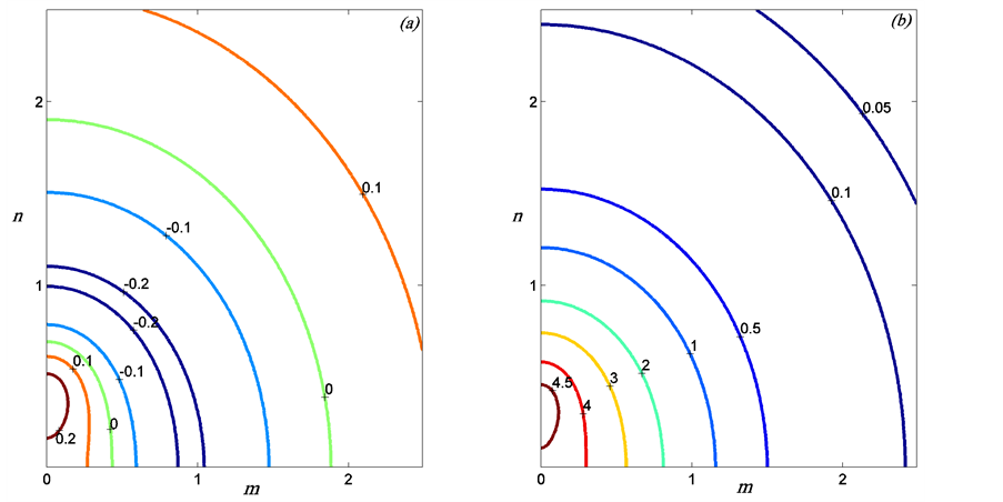
Figure 4. The contours of the discriminant,  , in the
  plane when
 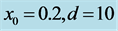 for two different values of
 : (a)
: (a)  and (b)
 .
.  here is scaled by
  for ease of presentation. Note that a region of negative values of the discriminant appears when the plume is close to the wall as in (a), which indicates instability of the plume at zero order.
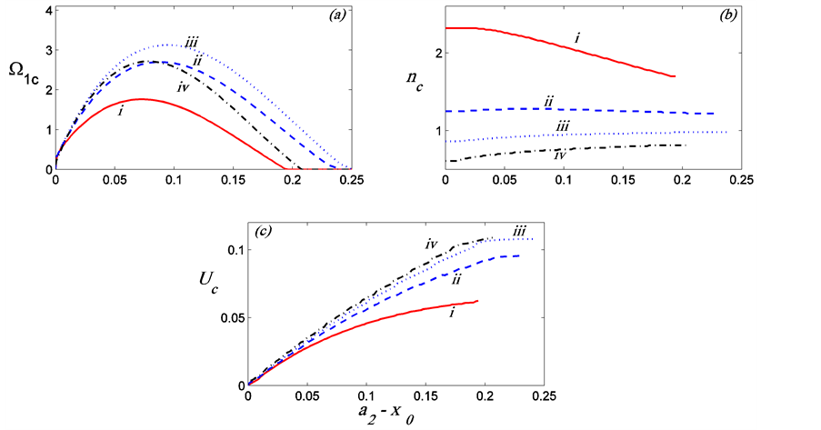
Figure 5. The preferred mode of instability with growth rate of order  as a function of the distance from the sidewall,
  , for four different values of
 ;
;  = 0.1,
  = 0.2,
  = 0.3 and
  = 0.4, when
 . Note the dependence of the magnitude of the growth rate on the thickness of the plume and its distance from the wall.
This instability with growth rate  occurs only if the plume is relatively thin (of thickness not more than about half the salt-finger length scale) and its distance from the sidewall does not exceed about 0.25. We also note that when the plume is very close to the wall the growth rate becomes smaller.
The preferred mode is associated with plume interfaces that are determined by (39) and (41). The amplitude at
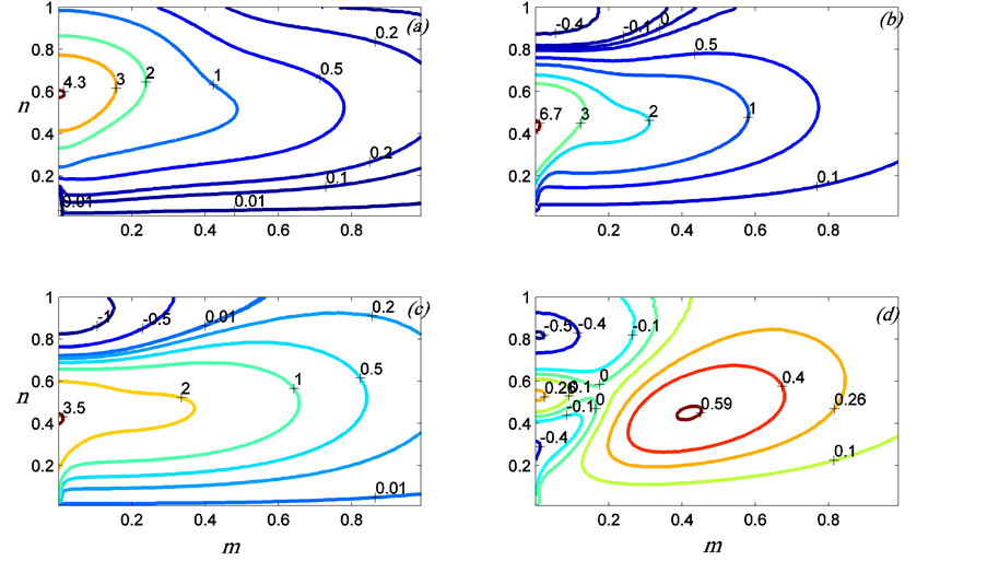
Figure 6. Contours of the growth rate of the modes MV, as in (a) and (c), and MS, as in (b) and (d), in situations when the preferred mode changes from one type to another. Here ,
,  , and
, and , and
, and  for (a), (b) and
  for (c), (d). (a), (c) refer to the MV mode and (b) , (d) refer to the MS mode. Note that the MS mode is preferred for
  and the MV mode is preferred when
 .
.
Figure 7. Illustration of the influence of the sidewalls on the stability of the Cartesian plume. The preferred mode as a function of Prandtl number,  , when
  and the plume is situated halfway between the sidewalls (i.e.,
 ). The curves i and ii refer to two different distances between the sidewalls: i)
 , and ii)
 . The solid curve refers to the MS mode while the broken one refers to the MV mode. Note the decrease in the growth rate as the distance
  between the sidewalls is reduced. The presence of the boundaries also decreases the range of
  for which the MS mode is preferred.
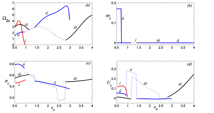
Figure 8. The preferred mode parameters as a function of  for
for  and
and  for three different values of
 : (i) 1, (ii) 3, (iii) 5. The solid curve refers to the MS mode while the broken one refers to the MV mode. The modes are two-dimensional except in the case of thin plumes when
 . Note the complicated behaviour of the preferred mode as the thickness of the plume changes at different positions relative to the boundaries.
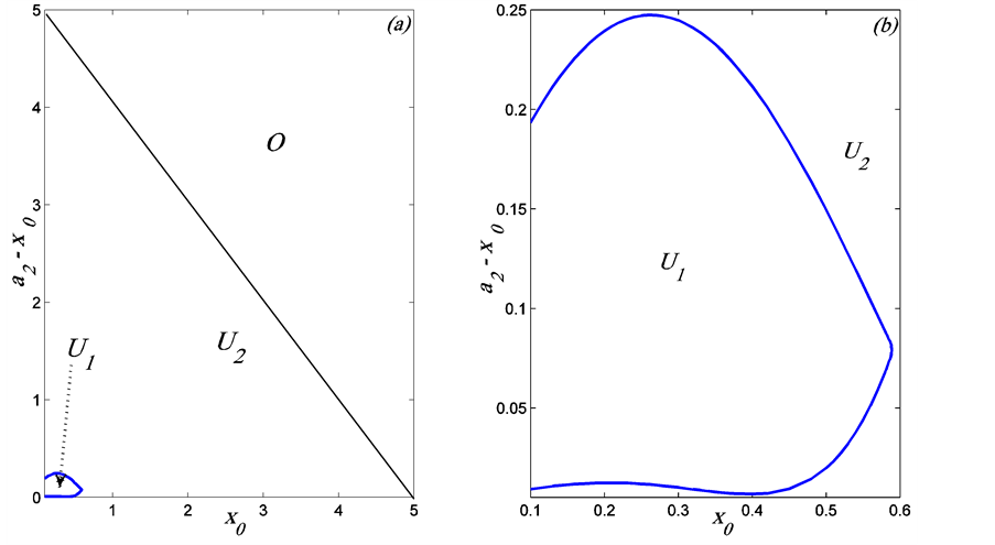
Figure 9. The regime diagram of the bounded Cartesian plume in the plane  for fixed
 . In (a), the regions labelled
  and
and  refer to instabilities with growth rate
  and
and , respectively. The area
  is outside the domain since cannot exceeds. Subfigure (b) shows a magnification of thearea for
 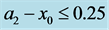 and
and  of figure (a).
 is fixed at the value 1 while the amplitude at the interface at
  is determined by
 , which is
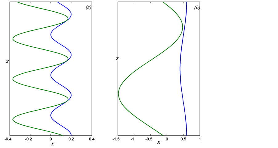
Figure 10. A sample of the profiles of the interfaces of the unstable mode for two values of the pair  when
when . The profiles are magnified for clarity by the same factor
 . (a)
. (a) ,
,  ,
,  and (b)
 ,
,  ,
, . Note that the interface profiles are very close at regular intervals.
determined by the parameters of the preferred mode for any prescribed values of . In figure 10 we give samples of the profiles of the interfaces relating to some preferred modes. It is noteworthy that the interfaces are very close at regular points across the length of the plume and this may indicate a tendency to break into blobs.
6. Conclusions
The dynamics of a plume of buoyant fluid, in the form of a channel of finite width, rising in a less buoyant fluid contained between two parallel sidewalls, a distance  apart, has been investigated. It is found that:
1) The plume is associated with a vertical flow that is balanced by a down flow on either side of the plume, and the flow inside the plume can develop a reverse (downward) flow around the center of the plume if the plume is wide enough.
2) The flow and concomitant temperature transport material upwards and heat downwards in such a way that the net upward buoyancy flux is positive, and possesses two local maxima and a minimum.
3) The instability of the interfaces has the following main properties:
a) The instability can take one of two modes, which are modifications of the sinuous and varicose modes of the plume in the absence of sidewalls but here modified by the lack of symmetry due to the different positions of the plume relative to the sidewallsb) If the plume is close to a sidewall, the instability has a growth rate  on the convective time scale, provided
  does not exceed a certain valuec) For plumes away from the sidewalls, the instability has a growth rate of
 d) The presence of the boundaries tend to stabilise the plume when it is equidistant from the sidewalls and the growth rate of the unstable mode is reduced as the sidewalls approach the plumee) When the Prandtl number is small, the modified sinuous (MS) mode is preferred while the modified varicose (MV) mode is preferred for large values of the Prandtl numberf) The preferred MS mode is generally 3-dimensional while the MV mode is generally 2-diemnsionalg) The profiles of the unstable plume indicate that the instability might lead to the break-up of the plume into blobs that rise to the top.
4) The relatively large growth rates of the instability when the plume is close to a sidewall may be due to heat flux emitted by the boundary.
The role of diffusion has been neglected in the present study because it is generally very small. However, it can be expected that it maybe potent when the plume is close to a sidewall. This has been analysed (but not included here) and found to provide small correction. Diffusion may also be potent in thin boundary layers at the interfaces of the plume at , where the concentration profile experiences a jump. This is expected to be analysed in a future study.
An attempt was made to compare the present results with experimental observations but we have not been able to identify a detailed experimental study on the influence of the boundaries on the plumes rising from mushy layers. However, the results obtained here agree with the general observations of Hell a well et al. [14] .
References
References
Rees Hones, D.W. and Worster, M.G. (2013) Fluxes through Steady Chimneys in a Mushy Layer during Binary Alloy Solidification. Journal of Fluid Mechanics, 714, 127-151. http://dx.doi.org/10.1017/jfm.2012.462
Wells, A.J. Wettlaufer, J.S. and Orszag, S.A. (2011) Brine Fluxes from Growing Sea Ice. Geophysical Research Letters, 38, Article ID: L04501. http://dx.doi.org/10.1029/2010GL046288
Loper, D.E. (1978) The Gravitationally Powered Dynamo. Geophysical Journal International, 54, 389-404. http://dx.doi.org/10.1111/j.1365-246X.1978.tb04265.x
Moffatt, H.K. (1989) Liquid Metal MHD and the Geodynamo. In: Lielpeteris, J. and Moreau, R., Eds., Liquid Metal Magnetohydrodynamics, Kluwer Academic Publishers, Dordrecht, 403-412. http://dx.doi.org/10.1007/978-94-009-0999-1_49
Al-Lawatia, M.A. Elbashir, T.B.A., Eltayeb, I.A., Rahman, M.M. and Balakrishnan, E. (2011) The Dynamics of Two Interacting Compositional Plumes in the Presence of a Magnetic Field. Geophysical & Astrophysical Fluid Dynamics, 105, 586-615. http://dx.doi.org/10.1080/03091929.2010.518316
Copley, S.M. Giamel, A.F., Johnson, S.M. and Hornbecker, M.F. (1970) The Origin of Freckles in Unidirectionally Solidified Casting. Metallurgical Transactions, 1, 2193-2204. http://dx.doi.org/10.1007/BF02643435
Huppert, H.E. (1990) The Fluid Mechanics of Solidification. Journal of Fluid Mechanics, 212, 209-240. http://dx.doi.org/10.1017/S0022112090001938
Chen C.F. and Chen, F. (1991) Experimental Study of Directional Solidification of Aqueous Ammonium Chloride Solution. Journal of Fluid Mechanics, 227, 567-586. http://dx.doi.org/10.1017/S0022112091000253
Tait S. and Jaupart, C. (1992) Compositional Convection in a Reactive Crystalline Mush and Melt Differentiation. Journal of Geophysical Research, 97, 6735-6756. http://dx.doi.org/10.1029/92JB00016
Jellinek, A.M. Kerr, R.C. and Griffiths, R.W. (1999) Mixing and Compositional Stratification Produced by Natural Convection: 1. Experiments and Their Application to Earth’s Core and Mantle. Journal of Geophysical Research, 104, 7183-7201. http://dx.doi.org/10.1029/1998JB900116
Classen, S. Heimpel, M. and Christensen, U. (1999) Blob Instability in Rotating Compositional Convection. Geophysical Research Letters, 26, 135-138. http://dx.doi.org/10.1029/1998GL900227
Aussillous, P. Sederman, A.J., Gladden, L.F., Huppert, H.E. and Worster, M.G. (2006) Magnetic Resonance Imaging of Structure and Convection in Solidifying Mushy Layers. Journal of Fluid Mechanics, 522, 99-125. http://dx.doi.org/10.1017/S0022112005008451
Pol, S. Fernando, H.J.S. and Webb, S. (2010) Evolution of Double Diffusive Convection in Low-Aspect Ratio Containers. American Physical Society, 55, 81.
Hellawell, A. Sarazin, J.R. and Steube, R.S. (1993) Channel Convection in Partly Solidified Systems. Philosophical Transactions of the Royal Society A, 345, 507-544. http://dx.doi.org/10.1098/rsta.1993.0143
Eltayeb I.A. and Loper, D.E. (1991) On the Stability of Vertical Double-Diffusive Interfaces. Part 1. A Single Plane Interface. Journal of Fluid Mechanics, 228, 149-181.
Eltayeb I.A. and Loper, D.E. (1994) On the Stability of Vertical Double-Diffusive Interfaces. Part 2. Two Parallel Interfaces. Journal of Fluid Mechanics, 267, 251-271. http://dx.doi.org/10.1017/S0022112094001175
Eltayeb I.A. and Loper, D.E. (1997) On the Stability of Vertical Double-Diffusive Interfaces. Part 3. Cylindrical Interfaces. Journal of Fluid Mechanics, 353, 45-66. http://dx.doi.org/10.1017/S0022112097007374
Eltayeb, I.A. (2006) The Stability of a Compositional Plume Rotating in the Presence of a Magnetic Fluid. Geophysical & Astrophysical Fluid Dynamics, 100, 429-455. http://dx.doi.org/10.1080/03091920600799541
Appendix A: Derivation of the Expression for the Growth Rate of the Cartesian Plume
Here we derive the solvability condition for the first order system (i.e., problem 1) in order to obtain an expression for the growth rate . Elimination of all variables
  and
and  from equations (97)-(99) in favor of
  gives
gives
 (A.1)
(A.1)
in which  is defined by
 (A.2)
(A.2)
Next, we consider a function  satisfying the homogeneous form of (95)
 (A.3)
(A.3)
and satisfies the following conditions
 (A.4)
(A.4)
 (A.5)
(A.5)
 (A.6)
(A.6)
It then follows that
 (A.7)
(A.7)
where  and
and  are given by
 (A.8)
(A.8)
 (A.9)
(A.9)
and  refers to the modes MS and MV. We now multiply equation (95) by
 , integrate by parts from
  to
to , and use the conditions for
 ,
,  and
and  at the interfaces and the boundaries to obtain
 (A.10)
where  and
and  are defined by
 (A.11)
Now we define a function  by
by
 (A.12)
and introduce the function
 (A.13)
and note that
 (A.14)
and
 (A.15)
 (A.16)
where  and
and  are defined by (A.8) and (A.9), while
  and
and  are similarly defined by
 (A.17)
 (A.18)
We multiply equation (A.1) by  and integrate from
  to
to , noting that
  and
and  satisfy the equations
 (A.19)
and have the proprieties
 (A.20)
 (A.21)
 (A.22)
 (A.23)
to obtain the relation
 (A.24)
where  is defined in (112) and
  and
and  are given by
 (A.25)
 (A.26)
We now eliminate the integral involving  between (A.10) and (A.24) to obtain an expression for
 (A.27)
which is the expression for the growth rate in terms of the zeroth order variables and the basic state only.