Open Journal of Applied Sciences
Vol.06 No.01(2016), Article ID:63156,14 pages
10.4236/ojapps.2016.61007
A Spatial Evapotranspiration Tool at Grid Scale
Sivarajah Mylevaganam*, Chittaranjan Ray
University of Nebraska-Lincoln, Lincoln, NE, USA

Copyright © 2016 by authors and Scientific Research Publishing Inc.
This work is licensed under the Creative Commons Attribution International License (CC BY).
http://creativecommons.org/licenses/by/4.0/


Received 21 December 2015; accepted 25 January 2016; published 28 January 2016
ABSTRACT
The drastic decline in groundwater table and many other detrimental effects in meeting irrigation demand, and the projected population growth have force to evaluate consumptive use or evapotranspiration (ET), the rate of liquid water transformation to vapor from open water, bare soil, and vegetation, which determines the irrigation demand. As underscored in the literature, Penman-Monteith method which is based on aerodynamic and energy balance method is widely used and accepted as the method of estimation of ET. However, the estimation of ET is oftentimes carried out using meteorological data from climate stations. Therefore, such estimation of ET may vary spatially and thus there exists a need to estimate ET spatially at different spatial or grid scales/resolutions. Thus, in this paper, a spatial tool that can geographically encompass all the best available climate datasets to produce ET at different spatial scales is developed. The spatial tool is developed as a Python toolbox in ArcGIS using Python, an open source programming language, and the ArcPy site-package of ArcGIS. The developed spatial tool is demonstrated using the meteorological data from Automated Weather Data Network in Nebraska in 2010.
Keywords:
Evapotranspiration, Penman-Monteith Method, Aerodynamic Method, Energy Balance Method, Python, ArcPy, ArcGIS, Spatial Scale, Geoprocessing, Python Toolbox

1. Introduction
The world population is projected to grow from 6.9 billion in 2010 to 9.1 billion in 2050 [1] . With this projected population growth, it has been documented that by 2050 the food demand is expected to increase by 70% [2] . Having said this, as per the ongoing evaluation by [1] , the current status of food scarcity is not at a level to appreciate or sustain, specifically in developing countries. Therefore, for the next few decades, the most striking focus would be on food security to meet the growing demand. With this statement in mind, to alleviate global hunger and to improve food security in the world, many initiatives and collaborations at global levels have been taken up to ensure availability of adequate food supply by means of efficient use of resources. One of the key limited resources that influences the definition of food security is the available freshwater [1] [2] .
Although over 70% of Earth’s surface is covered by water, the amount of freshwater available for appropriation is limited as 97.5% of all water on Earth is saline [3] . This limited freshwater is competed by many water users such as irrigation, household and municipal, and industrial. Among these water users, irrigation demand accounts for 87% of the total use globally [1] [2] . The consequences of such high demand on irrigation in addition to the demands from other water users have forced to pump water heavily from groundwater aquifers. This has arguably caused groundwater tables to decline in many regions, including in Afghanistan, China, India, Iran, Pakistan, and the US. The drastic decline in groundwater table and many other detrimental effects in meeting irrigation demand, and the projected population growth have force to evaluate the consumptive use or evapotranspiration (ET), the rate of liquid water transformation to vapor from open water, bare soil, and vegetation, which determines the irrigation demand.
As underscored in the literature [4] -[8] , to date, there are many methods available to estimate ET. These methods are either empirical or climate data driven. Under empirical based estimation of ET, Blaney-Criddle method or its modified version is widely used in the arid western regions of the United States [4] [5] . However, this method doesn’t account for humidity, wind speed, and other climate factors. On the other hand, using meteorological data from climate stations, the methods of estimation of ET include aerodynamic method, energy balance method, and combination methods such as Penman-Monteith method [4] -[6] . The aerodynamic method of determining evaporation considers the transport of water vapor by the turbulence of the wind blowing over a natural surface. The energy balance method considers all heat energy received and reflected/dissipated by a cropped area or a water body. Penman-Monteith method of evaporation is obtained by combining the evaporation computed by aerodynamic and energy balance method [6] . The weighting factors are applied in combining the methods (i.e., aerodynamic and energy balance). The weighting factors account for aerodynamic resistance and surface resistance that accounts for movement of water vapor from the plant leaves to the atmosphere. As underscored in the literature [4] -[8] , Penman-Monteith method is widely used and accepted as the method of estimation of ET. However, the application using Penman-Monteith is oftentimes evaluated using meteorological data from climate stations.
The current practices of water resources planning and management are at watershed scale and oftentimes at grid scale in parallel with the contemporary technology development. Having said this, as discussed previously, the estimation of ET is carried out using meteorological data from climate stations. However, such estimation of ET may vary spatially and thus there exists a need to estimate ET spatially. Moreover, in the absence of optimum spatial scale, and with a growing interest of watershed studies at different spatial scales [9] , the need to evaluate the variation of ET at different spatial scales is also required. Thus, in this paper, a spatial tool that can geographically encompass all the best available climate datasets to produce ET at different spatial scales is developed using Python, an open source programming language supported by a growing user community for its extensive collection of standard and third-party libraries, and the ArcPy site-package of ArcGIS.
2. Estimation of Evapotranspiration
The need to manage the available freshwater wisely with ever increasing population and the demand from irrigation has brought ET as one of the critical subject areas to research in the field of hydrology. Over the years, with many research works, numerous methods have been developed to estimate ET. These methods mainly fall under these categories: 1) aerodynamic method, 2) energy balance method, and 3) combination of aerodynamic and energy balance methods.
2.1. Aerodynamic Method
This method of determining evaporation considers the transport of water vapor by the turbulence of the wind blowing over a natural surface. According to this method, the evaporation , generally from lakes and reservoirs, is proportional to
 . The mathematical expression of this method is given by Equation (1).
 (1)
(1)
where M,  , and
, and  are mass transfer coefficient, saturated vapor pressure at water temperature, vapor pressure at height z, and wind velocity at height z, respectively. The mass transfer coefficient is given by Equation (2).
 (2)
(2)
where , and
, and  are atmospheric pressure at height z, density of water, density of air, and evaporation coefficient, respectively.
By substituting Equation (2) in Equation (1),
 (3)
(3)
Considering aerodynamic resistance,  , Equation (3) leads to
 (4)
(4)
Since , Equation (4) becomes
 (5)
(5)
where T is the air temperature in degree Celsius.
 (5’)
(5’)
2.2. Energy Balance Method
As shown in Figure 1, this method considers all heat energy received and reflected/dissipated by a cropped area or a water body. The portion of energy that is used to warm the air in contact with the ground or water surface is known as sensible heat flux (H). The term G is the heat conduction from the water surface or soil to the layer of soil or water below. Since the energy required to evaporate a unit mass of water is called latent heat of vaporization (λ), the total energy absorbed per unit area to evaporate  is
is . Therefore, neglecting the other small energy terms that are dissipated/stored, the energy balance for the control volume shown in Figure 1 is given by Equation (6).
 (6)
(6)
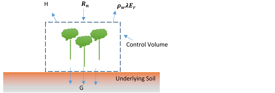
Figure 1. The energy flow diagram for a cropped area.
where  is the net radiation. The latent heat of vaporization is 2.45 MJ/kg at about 20 degree Celsius [6] . However, to account for temperature variation, the latent heat of vaporization is given by
 (6’)
(6’)
The sensible heat flux defined by Equation (7) is related to Bowen ratio, 
 (7)
(7)
Bowen ratio,  is derived from temperatures and vapor pressures at two heights above the water
surface. By substituting Equation (7) in Equation (6),
 (8)
(8)
Since ,
,
 (9)
(9)
As shown in Equation (10), the net radiation  is the sum of net long-wave radiation
  and net short-wave radiation
 .
.
 (10)
(10)
The net short-wave radiation that is defined by Equation (11) is a function of total extraterrestrial radiation
 and cloudiness fraction
 .
.
 (11)
(11)
The net long-wave radiation which is in accord with Stefan-Boltzmann’s law of black body radiation is given by Equation (12).
 (12)
(12)
where , and T are vapor pressure at air temperature, Stefan-Boltzmann constant, and mean air temperature, respectively.
2.3. Combination Method of Penman
As shown in Equation (13), this method of evaporation is obtained by combining the evaporation computed by
aerodynamic  and energy balance method
 . The weighting factors (i.e.,
  and
and ) are
) are
applied in combining the methods (i.e., aerodynamic and energy balance). The weighting factors sum to unity.
 (13)
(13)
where  is the psychrometric constant that is defined by Equation (14). The gradient of the saturated vapor pressure
  is given by Equation (15).
 (14)
(14)
 (15)
(15)
2.4. Penman-Monteith Method
This method is same as the combination method of Penman. However, in this method, similar to , another term called surface resistance
  is introduced to account for resistance associated with movement of water vapor from the plant leaves to the air outside. This method is widely used to estimate evapotranspiration. The mathematical expression of this method is given by Equation (16).
 (16)
(16)
For grass reference crop,  and
and . Therefore, for grass reference crop
 .
.
where  is the wind speed at 2 m. When the wind speed is measured at different elevation, it can be adjusted from one level to another by using Equation (17).
 (17)
(17)
where Z1, Z2 are measurement heights for levels 1 and 2, respectively. Z0 is the reference height where velocity is zero. For open agricultural area, Z0 = 0.03.
3. The Development of Spatial Evapotranspiration Tool (SET) at Grid Scale
ArcGIS provides easy-to-use platform to extend its desktop features by accessing geoprocessing functionalities through programming/scripting languages. Python, an open source programming language supported by a growing user community for its extensive collection of standard and third-party libraries, is one of the scripting languages supported by Environmental Systems Research Institute (Esri). The communication between ArcGIS and Python is through a site-package that is called ArcPy. The ArcPy site-package encompasses the modules, functions, and classes required to access the geoprocessing functionalities. The modules are the main gates to access the geoprocessing functionalities. The ArcPy site-package comes with a series of modules such as data access module, mapping module, and ArcGIS Spatial Analysis Extension module. To support the main modules, the ArcPy site-package also has some classes that are oftentimes used as shortcuts to complete geoprocessing parameters. Using the ArcPy site-package, the customization of desktop features could be in three ways: desktop add-in, standard toolbox, and Python toolbox.
3.1. Python Desktop Add-In
To extend desktop functionality, in ArcGIS 10, a new desktop add-in model that are authored using .NET or JAVA programming languages was introduced. The extension of functionality could be to make a customization that performs an action in response to an event such as dragging a rectangle over a geographical map to define an area of interest. This new add-in model is further enhanced by introducing Python to the list of supported programming languages, and the Python add-in wizard to reduce the development effort.
3.2. Standard and Python Toolboxes
ArcGIS tools that are boxed within toolboxes are a chunk of codes used to perform small, but essential tasks on geographical data. ArcGIS with its installation comes with a set of tools that are known as system tools. Oftentimes, geographic information system (GIS) professionals are required to repeat a task again and again by using one or more of the system tools. To facilitate this, a script is written using Python scripting language and the ArcPy site-package. This script is then attached to a newly created toolbox. The newly created toolbox could be either a standard or Python toolbox. In case of Python toolbox, which is an ASCII-based file, the toolbox is created entirely in Python.
Since the development of SET at grid scale does not involve an event such as dragging a rectangle over a geographical map to define an area of interest, Python toolbox is used to develop the SET.
3.3. The Spatial Evapotranspiration Tool (SET) at Grid Scale
The skeleton of ArcGIS Python toolbox is basically a class in Python. A toolbox can have more than one tool. Each tool is defined by a Python class. The tools are associated with the toolbox class by setting the “tools” property of the toolbox within the constructor or the class initialization method of the toolbox class. For example, in the below shown code, a tool named “SpatialET” is associated with the toolbox. The “label” and the “alias” are the properties of the toolbox, which are used in calling the tool in geoprocessing tasks.
class Toolbox(object):
def __init__(self):
self.label = "Spatial Evapotranspiration"
self.alias = "grid"
self.tools = [SpatialET]
class SpatialET(object):
def __init__(self):
…
def getParameterInfo(self):
…
defisLicensed(self):
defupdateParameters(self, parameters):
defupdateMessages(self, parameters):
def execute(self, parameters, messages):
…
The constructor or the class initialization method of Spatial ET class is used to set the properties of the tool. The “label” and “description” are the most important properties. The “canRunInBackground” property is used to let the tool to run in the background. As shown below, For SET, this property is set to “False”.
class SpatialET(object):
def __init__(self):
self.label = "SpatialET"
self.description = "This tool is about Evapotranspiration at grid scale."
self.canRunInBackground = False
Within the Spatial ET class, the method named getParameterInfo() is used to collect the user specified inputs such as the location of raster data of temperature, relative humidity, wind speed, and solar radiation. These inputs are used to calculate ET using Penman-Monteith at grid scale. Within the getParameterInfo(), the parameter() object is used to collect each input from the user. For example, as shown in the below code, the variable named “param0” is used to collect the location of raster data of temperature. The parameter() object has few properties such as name, datatype, parametertype, and direction. Since the user input for the temperature is a raster, the datatype of param0 is set to “DERasterDataset”. Furthermore, the temperature raster dataset is an input. Therefore, the direction property of “param0” is set to “Input”. This same chunk of code is repeated for the other inputs (e.g., solar radiation, relative humidity, and wind speed) collected from the user through the tool.
def getParameterInfo(self):
param0 = arcpy.Parameter(
displayName="Temperature",
name="Temperature_raster",
datatype="DERasterDataset",
parameterType="Required",
direction="Input")
After collecting the parameters, they are stored within a list as shown in the below code, where param0, param1, param2, param3, param4, and param5 are the variables used to store the temperature raster, relative humidity raster, wind speed raster, location of tool generated ET raster, wind speed measurement height, and solar radiation raster, respectively. The default wind speed measurement height is also set to 3 m. This list is returned from getParameterInfo() method. The graphical user interface of the above outlined code is shown in Figure 2.
params = [param0,param1,param2, param3, param4, param5]
params[4].value=3
return params
Since the developed tool is in need of spatial analyst extension, the isLicensed()methodis used to check the existence of required licenses. The updateMessages() and updateParameters() are some of the other methods that could be used to customize the tool further. In SET, these methods are not modified as it doesn’t require customization using these methods.
def isLicensed(self):
return True
After having stored the information on user specified inputs, the execute() method of the tool is used to setup the Penman-Monteith method as discussed in section 2.0. One of the arguments of the execute() method is “parameters” that has all the input data obtained through getParameterInfo() method. This argument is a list. Therefore, the individual inputs are retrieved using the indices of the list and the valueAsText() method of the parameter object. For example, as shown below, to retrieve the temperature raster, the zeroth index of the list is called. This procedure is followed to retrieve the other inputs as well. Since the user specified temperature raster is in ˚F, a temporary raster of temperature in ˚C is created and stored in the Python variable named “inRasterTempC”.

Figure 2. The graphical user interface of SET.
#User inputs for the tool
inRasterTempF=parameters[0].valueAsText #Temp
inRasterRH=parameters[1].valueAsText #RH
inRasterW=parameters[2].valueAsText #Wind speed
outRaster1=parameters[3].valueAsText # The name of the ET Raster
inWindHeight=parameters[4].value # Anero height
inSolarRadiation=parameters[5].valueAsText # So
inRasterTempC=(Raster(inRasterTempF)-32)/1.8
Within the execute() method, raster operations are carried out using the syntax of Map Algebra. As shown below, the raster of saturated vapor pressure is developed using the user specified temperature raster. The developed raster of saturated vapor pressure is multiplied by the raster of relative humidity to get the raster of vapor pressure. This is a raster operation. In other words, ArcGIS generates values for each grid based on the respective raster values of saturated vapor pressure and the relative humidity. This can be further explained as shown in Figure 3.
outSaturated=0.6108*Exp((inRasterTempC*17.27)/(237.3+inRasterTempC)) #Saturated vapor pressure
outSaturatedZ=outSaturated*Raster(inRasterRH)/100 #Vapor pressure
The developed rasters are temporary. In other words, they are not physically stored in a specified location. These temporary rasters are used in the subsequent raster operations to develop the other temporary rasters associated with Penman-Monteith method. The detailed raster operations in computing ET using Penman-Monteith method is outlined in Figure 4.
To calculate the ET using energy balance method, two inputs at grid levels are required: the latent heat of vaporization and the net radiation which is the sum of net long wave and net short wave radiation. As shown in the below code, the latent heat of vaporization is developed at grid level using equation (6’). The net radiation raster that is named “NetRadiation” is also developed to produce the raster of ET using energy balance method at grid scale.
outLamda=2.501-0.002362*inRasterTempC #Latent heat of vaporization
NetSRadiation=(1-0.23)*(0.25+0.5*0.25)*Raster(inSolarRadiation)#Net SW Radiaition
NetLRadiation=-1*(0.1+0.9*0.25)*(0.34-0.14*SquareRoot(outSaturatedZ))*(4.903/1000000000)*((273.2+ inRasterTempC)**4)
NetRadiation=NetLRadiation+NetSRadiation
EnergyBal=NetRadiation/1000/outLamda #Using energy balance method
Similarly, as shown in the below code, using raster operations and the temporary rasters, the ET using aerodynamic method is also developed. These raster operations are based on the equations discussed in section 2.0. The comments provided at each line explain the meaning of the variables.
Windspeed=Raster(inRasterW)
Windspeed2=0.44704*Windspeed*(Ln(2/0.03)/Ln(inWindHeight/0.03)) #Windspeed at 2m height
AerodynamicR=208/Windspeed2 #Aerodynamic resistance
inRasterP=1.225*(275+inRasterTempC)/3.486 #Pressure
PsychrConst=0.0016286*inRasterP/outLamda #Psychrometric constant
DeltaR=4098*outSaturated/((237.3+inRasterTempC)**2) #Vapor pressure gradient
AeroBal=2.17*(outSaturated-outSaturatedZ)/1000/AerodynamicR/(inRasterTempC+273)
#Using aerodynamic method

Figure 3. The computation of vapor pressure using raster operations at grid scale.
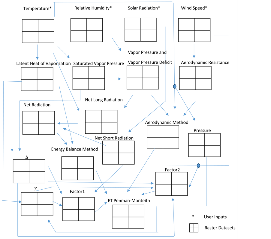
Figure 4. The raster operations in computing ET using Penman-Monteith.
The weights associated with each method (i.e., aerodynamic and energy balance method) are generated at grid scale. The weights are generated as per Equation (13). These weights are then applied to the computed ET using aerodynamic and energy balance to develop the raster of ET using the Penman-Monteith method. The developed raster is stored using the save() method of the raster, as per the user specified output name and the location.
Factor1=DeltaR/(DeltaR+PsychrConst*(1+0.33*Windspeed2)) #Factor for energy balance method
Factor2=PsychrConst/(DeltaR+PsychrConst*(1+0.33*Windspeed2)) #Factor for aerodynamic method
PenmanMon=(Factor1*EnergyBal+Factor2*AeroBal)*1000 #Evapotranspiration using Penman-Mon in mm/ day
PenmanMon.save(outRaster1)
4. The Application of SET
The state of Nebraska that lies in both the Great Plains and the Midwestern United States has a total geographical area of 200,520 km2. The total population of the state is 1.8 Million [10] . Both the surface and groundwater are used to meet the demand for wide range of purposes. Around 94.8% of the estimated total groundwater withdrawals is used to meet the irrigation demand [11] . As of November 2014, around 95,000 irrigation wells are registered in the state. The developed tool is demonstrated for the state of Nebraska using the meteorological data from Automated Weather Data Network (AWDN) that gathers climatological observational data and the information for High Plains Region and provides its shareholders in fields such as agriculture. Figure 5 shows the spatial locations of the climate stations in AWDN.
The AWDN has around 63 stations to cover the state of Nebraska. The data is available on hourly, daily, and sub-daily basis since 1985. To demonstrate the tool, the daily data in 2010 was downloaded from the online services provided by AWDN. As discussed in Section 3, the developed tool requires raster datasets on temperature, relative humidity, wind speed, and solar radiation. Therefore, at first, the average daily data in 2010 was developed based on the daily data of temperature, relative humidity, and wind speed. Using ArcGIS and the spatial locations of the climate stations, the tabular datasets of average daily data in 2010 were transformed to geographical data. Subsequently, the Spatial Analyst Extension of ArcGIS was used to develop the grid level values of temperature, relative humidity, and wind speed at a resolution of 1 km. The Kriging spatial interpolation technique packaged with ArcGIS was used to develop the rasters shown in Figure 6. To ensure that the Krigged data covers the whole state, the extent of the interpolation was set using the state map of Nebraska. The research work carried out by [4] was used to develop the solar radiation raster.
As depicted in Figure 6, in 2010, the temperature varies from 47˚F to 53˚F. The maximum temperature is observed in the Eastern part of Nebraska. The relative humidity that determines the vapor pressure is very high in the Eastern part of Nebraska and tends to decrease towards the Western part of the state. It is also worth to note that the trends of temperature and the wind speed are opposite. In other words, the wind speed tends to increase from Eastern part of Nebraska to Western part of Nebraska in the direction of South East to North West.
The estimated ET using Penman-Monteith method is shown in Figure 7(a). The Figure 7(b) shows the categorized version of Figure 7(a). For the state of Nebraska in 2010, the estimated ET using Penman-Monteith method varies from 0.77 to 1.04 mm/day. In other words, the maximum spatial variation of estimated ET using
Penman-Monteith method is . Moreover, the highest estimated
ET using Penman-Monteith method is registered in the Eastern part of Nebraska. However, the geographical extent of such high ET is limited to a very small area in contrast to the geographical area with estimated ET using Penman-Monteith method in the range of 0.77 - 0.96, as shown in Figure 7(b). Furthermore, an increasing trend of spatial variation is observed from Western part of Nebraska to Eastern part of Nebraska in the direction of North West to South East.

Figure 5. The spatial locations of the climate stations from AWDN Network in Nebraska.

Figure 6. The input rasters to SET: (a) The average daily temperature in 2010 in ˚F; (b) The average daily relative humidity in 2010 in %; (c) The average daily wind speed in 2010 in MPH; (d) The average daily solar radiation in MJm−2∙d−1.

Figure 7. The Estimation of ET (mm/day) using Penman-Monteith method.
Figure 8(a) and Figure 8(b) show the spatial variation of evapotranspiration estimated using energy balance method and the aerodynamic method, respectively.These figures reveal that the contribution of aerodynamic method for the estimation of ET using Penman-Monteith method is not that siginificant compared to that of energy balance method. In other words, the estimation of ET using Penman-Moneith is totally defined by the energy balance method. The lowest and the highest estimated ET using energy balance method is 2.3 mm/day and 2.44 mm/day, respectively. Therefore, the maximum spatial variation of estimated ET using energy balance
method is . Although the spatial variation of estimated ET using
energy balance method is not significant, an increasing trend of spatial variation is observed from Western part of Nebraska to Eastern part of Nebraska in the direction of North West to South East. Moreover, it is also important to note that even though the estimation of ET using Penman-Moneith is totally defined by the energy balance method, the spatial variation of estimated ET using Penman-Monteith method is not influenced by the energy balance method, but bythe weights used to determine the contribution of energy balance method.
On the other hand, The lowest and the highest estimated ET using aerodynamic method is  and
and , respectively. Therefore, the maximum spatial variation of estimated ET using aerody-
namic balance method is . In other words, the varia-
tion of estimated ET using aerodynamic method is spatially significant compared to that of energy balance method. Moreover, in contrast to what is observed with the trend of estimated ET using energy balance method, the lowest estimated ET using aerodynamic method occurs in the Eastern part of Nebraska and increases towards the Western part of Nebraska, as shown in Figure 8(b).
As shown in Figure 9(a), the weighting factor that is used to determine the contribution of energy balance
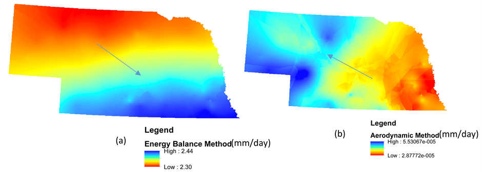
Figure 8. The estimation of ET (mm/day) using (a) Energy balance method and (b) Aerodynamic method.

Figure 9. Weighting factor for (a) Energy balance method and (b) Aerodynamic method.
method on estimation of ET using Penman-Monteith ranges from 0.34 to 0.43. Similarly, as shown in Figure 9(b), the weighting factor that is used to determine the contribution of aerodynamic method on estimation of ET using Penman-Monteith ranges from 0.29 to 0.32. In other words, in addition to the fact that the contribution of aerodynamic method on estimation of ET using Penman-Monteith is very small, the weighting factor that is used to determine the contribution of aerodynamic method is smaller than weighting factor that is used to determine the contribution of energy balance method. Furthermore, it is also noted that the weighting factor that is used to determine the contribution of energy balance method tends to follow the same trend as in Figure 8(a). In other words, higher ET estimated using energy balance method is weighted more and lower ET estimated using energy balance method is weighted less. In contrast to this, in the case of aerodynamic method, higher ET estimated using aerodynamic method, although the value is very small, is weighted less and lower ET estimated using aerodynamic method is weighted more. This is notable from Figure 8(b) and Figure 9(b).
5. Conclusion and Recommendations
In this paper, a spatial tool that can geographically encompass all the best available climate datasets to produce ET using Penman-Monteith method at different spatial scales is developed using Python, an open source programming language supported by a growing user community for its extensive collection of standard and third- party libraries, and the ArcPy site-package of ArcGIS. The developed spatial tool is demonstrated using the meteorological data from Automated Weather Data Network (AWDN) in Nebraska in 2010. Based on the development and demonstration of the tool, the following points are highlighted:
1) The contribution of aerodynamic method for the estimation of ET using Penman-Monteith method is not that significant compared to that of energy balance method. However, the variation of estimated ET using aerodynamic method is spatially significant compared to that of energy balance method. In addition to the fact that the contribution of aerodynamic method on estimation of ET using Penman-Monteith is very small, the weighting factor that is used to determine the contribution of aerodynamic method is smaller than weighting factor that is used to determine the contribution of energy balance method on estimation of ET using Penman-Monteith.
2) It is also observed that even though the estimation of ET using Penman-Moneith is totally defined by the energy balance method, the spatial variation of estimated ET using Penman-Monteith method is not influenced by the energy balance method, but by the weights used to determine the contribution of energy balance method.
3) The demonstration of the developed tool was based on solar radiation raster from the work done by [4] . However, the solar radiation toolbox that is distributed with the installation of ArcGIS is an option that could be coupled with the developed tool.
4) In this study, the Kriging spatial interpolation scheme was used to transform the observed climate data from AWDN. Though Kriging is considered as one of the best spatial interpolation schemes, it is also worth to research on the impact of other interpolation schemes on spatial ET at grid scales. This may also lead to identify the impact of different schemes on energy balance method and the aerodynamic method on estimation of ET using Penman-Monteith.
5) Though the developed spatial tool is demonstrated for a spatial resolution of 1 km, it can be used to estimate ET using Penman-Monteith at different spatial resolutions to decide the best scale that fits a particular region or area, and to decide the impact of spatial resolutions on ET using Penman-Monteith.
6) The sensitivity of ET using Penman-Monteith is oftentimes estimated using meteorological data from climate stations. However, such estimation of sensitive or most influential parameters may vary spatially and thus there exists a need to estimate sensitivity of ET spatially. Thus, the developed tool will be of useful to research on this.
7) Though the developed spatial tool does not include the landuse datasets, the integration of one of the existing landuse datasets, such as the National Land Cover Database (NLCD) for the United States of America, with the tool is also worth to research.
Acknowledgements
The authors would like to thank the Board of Regents, University of Nebraska-Lincoln, Lincoln, for providing the financial support to conduct this research. This research was conducted when author* was a researcher at University of Nebraska-Lincoln, Lincoln.
Cite this paper
SivarajahMylevaganam,ChittaranjanRay, (2016) A Spatial Evapotranspiration Tool at Grid Scale. Open Journal of Applied Sciences,06,64-77. doi: 10.4236/ojapps.2016.61007
References
- 1. WWAP (World Water Assessment Programme) (2015) United Nations World Water Development Report 2015: Water for a Sustainable World. United Nations Educational, Scientific and Cultural Organization, Paris.
- 2. WWAP (World Water Assessment Programme) (2012) United Nations World Water Development Report 4: Managing Water under Uncertainty and Risk. United Nations Educational, Scientific and Cultural Organization, Paris.
- 3. Postel, S.L., Daily, G.C. and Ehrlich, P.R. (1996) Human Appropriation of Renewable Fresh Water. Science, 271, 785- 788. http://dx.doi.org/10.1126/science.271.5250.785
- 4. Jensen, M.E., Burman, R.D. and Allen, R.G. (1990) Evapotranspiration and Irrigation Water Requirements, Manuals and Reports on Engineering Practice. ASCE No. 70, New York.
- 5. Richard, G.A. and William, O.P. (1986) Rational Use of the FAO Blaney-Criddle Formula. Journal of Irrigation and Drainage Engineering, 112, 139-155. http://dx.doi.org/10.1061/(ASCE)0733-9437(1986)112:2(139)
- 6. Allen, R.G., Pereira, L.S., Raes, D. and Smith, M. (1998) Crop Evapotranspiration-Guidelines for Computing Crop Water Requirements. FAO Irrigation and Drainage Paper 56, United Nations Food and Agriculture Organization, Rome.
- 7. Gong, L.B., Xu, C.Y., Chen, D.L., Halldin, S. and Chen, Y.Q.D. (2006) Sensitivity of the Penman-Monteith Reference Evapotranspiration to Key Climatic Variables in the Changjiang (Yangtze River) Basin. Journal of Hydrology, 329, 620-629. http://dx.doi.org/10.1016/j.jhydrol.2006.03.027
- 8. Bakhtiari, B. and Liaghat, A.M. (2011) Seasonal Sensitivity Analysis for Climatic Variables of ASCE Penman-Monteith Model in a Semi-Arid Climate. Journal of Agricultural Science and Technology, 13, 1135-1145.
- 9. Kevin, F.D., Thomas, E.R. and William, L.C. (2015) Groundwater Availability in the United States: The Value of Quantitative Regional Assessments. Hydrogeology Journal, 23, 1629-1632. http://dx.doi.org/10.1007/s10040-015-1307-5
- 10. U.S. Census Bureau (2015) Annual Estimates of the Resident Population for the United States, Regions, States, and Puerto Rico: April 1, 2010 to July 1, 2014. U.S. Census Bureau, Suitland, Maryland.
- 11. Nebraska Surface Water and Groundwater Use—2005. Nebraska Department of Natural Resources. http://www.dnr.ne.gov/nebraska-surface-water-and-groundwater-use-2005
NOTES

*Corresponding author.