Open Journal of Applied Sciences
Vol.4 No.4(2014), Article ID:44228,13 pages DOI:10.4236/ojapps.2014.44021
Currency Areas: Public Debt, Inflation and Unemployment
Carlos Encinas-Ferrer
Faculty of Business, Universidad De La Salle Bajio, Leon, Mexico
Email: cencinas@delasalle.edu.mx
Copyright © 2014 by author and Scientific Research Publishing Inc.
This work is licensed under the Creative Commons Attribution International License (CC BY).
http://creativecommons.org/licenses/by/4.0/


Received 15 January 2014; revised 18 February 2014; accepted 26 February 2014
Abstract
Can public debt, inflation and unemployment tell us something about optimal or not optimal currency areas? In this paper, I compare the behavior of these variables in two countries, Mexico and the United States of America (USA), along with the member countries of the Euro Zone (European Monetary Union, or EMU). The main purpose is to know the divergence between public debt, average inflation −0% in the graphs—in the main cities or regions of the first two, and compare them with the countries of the EMU. The period of 2001-2012 is chosen to be the years in which the Euro has been circulating among member countries of the Monetary Union (EMU). We find significant differences that allow us to determine the faults that the criteria of divergence on these variables had on the founding treaty of the European Monetary Union.
Keywords
Currency Areas; Optimal Currency Areas; Nonoptimal Currency Areas; Public Debt; Inflation; Unemployment

1. Introduction
The economic and financial crisis that began in late 2007, called by several economists “The Great Recession”, has brought to the fore a discussion of economic policy clash between two great currents of the capitalist economic thought: Neoliberalism and Keynesianism.
It has also shown us that we lacked a general theory of currency areas and, therefore, elements that could allow us to determine with certainty, its characteristics as optimal or non-optimal.
As a product of this ignorance, the Treaty of Maastricht established a reduced number of requirements of convergence in some economic variables assuming that they were sufficient to give stability to the euro currency area. They led to a financial crisis which was supposed impossible just 12 years ago.
In this paper, I review what we know so far about currency areas and analyze three of these variables—public debt, inflation and unemployment, and the convergence criteria on them which were established at that Treaty.
2. Methodology
I carry out the comparison in the evolution of the chosen variables in two countries, Mexico and the United States of America (USA)—assuming they are optimal currency areas-along with the member countries of the Euro Zone (European Monetary Union, or EMU). The main purpose is to know the divergence between public debt, average inflation −0% in the graphs—in the main cities or regions if the first two, and compare them with the evolution of those variables in the countries of the EMU. The period of 2001-2012 is chosen to be the years in which the Euro has been circulating among member countries of the Monetary Union (EMU).
3. Discussion
What do we mean when we talk about a currency area? This is a question that until now I have started to make me and despite the fact that many years ago I read the famous paper of Robert A. Mundell, “A Theory of Optimum Currency Areas” [1] , and in 2009 I wrote the article “Analysis of the balance of payments under dollarization: Toward a theory of nonoptimal currency areas” [2] .
Before defining the optimum or not of a monetary zone or area we should explain what we mean by it. However, when we look for a definition of what is a currency area we find that almost all them are accompanied by the adjective “optimal”. It seems that all assume something but do not tell us what.
A currency area may be a single country or necessarily we are referring to a number of them? A currency area is a region comprising several countries with a single currency circulating, as in Europe, or is one in which several currencies do but with the predominance of one of them? Does the United States of America (USA) and Ecuador form a currency area?
Mundell defined a currency area as a territory within which exchange rates are fixed. Does this involve several countries and different currencies? Our author speaks of the difference between a currency area that has a single currency and a currency area comprising several coins and in the first case seems to refer to a single country with a central bank. It is obvious that in 1961 nobody could glimpse that the prevailing exchange rates were flexible and “it hardly appears within the realm of political feasibility that national currencies would ever be abandoned in favor of any other arrangement” as Mundell himself writes in his famous article. But the fact is we do not see a clear definition of monetary area.
Samuelson and Nordhaus [3] however point out that most economists believe the United States of America is an optimum currency area. This would imply that this majority assumes that the country is a currency area and the word “believe” refers to the adjective “optimal”. I must clarify that I am worry about the verb “believe”.
In my article referred to at the beginning I defined a nonoptimal currency area as one that is formed when a country replaces unilaterally its own currency for another one, named “anchor currency”, and issued by a country or a currency union generally with high economic growth. As you can see, I was referring to as a nonoptimal currency area the country that replaces its own currency not to the issuer of the anchor currency.
Will I modify today that definition of nonoptimal currency area? Yes, I would, but incorporating not only those countries who replace their currencies unilaterally, but those countries that do it through a bilateral or multilateral monetary settlement with the lack of a broader economic policy, as happened with the European Monetary Union (EMU).
What I mean by broader agreements? Recent events in the Euro zone show us some of them: common policy in subjects such as fiscal policy, public debt, bank regulation and deposit insurance, among others.
In the case of public debt, incorporating the concept of potential debt, referring not only to regional, state and provincial as well as local debts, but also the bad bank debts that become debt at high speed, as we saw in Mexico in 1995 and 1996, and currently in Ireland, Greece, Spain and more recently in Cyprus, plus those other economies still missing.
Returning to the original subject, it would seem that in economics it has been assumed that an optimum currency area is made up of several nations that work as a country, trying to extrapolate its characteristics to the whole. If so, let me disagree and point out that a country can also be a nonoptimal currency area something that will be worth analyzing in other research.
Up to the moment my analysis of this issue has led me to the following conclusions:
1) A currency area can be both a country and a number of them with a single currency that functions similarly to how a single nation does.
2) A currency area can refer also to a group of countries with different currencies in which one prevails over the other.
But this begs the question how does a nation monetarily work? How economic variables that are related to optimal monetary operation behave? In this paper we will refer to three of them: public debt, inflation and unemployment.
3.1. An Optimal Currency Area
First of all let’s try to find out what are the conditions that make an optimal currency area.
Robert Mundell, in his pioneer article mentioned at the beginning, emphasizes labor mobility between regions within the area: you won’t need as much a unified economic policy if unemployed people can move to where jobs are.
Ronald McKinnon [4] emphasizes the size of trade; with a big amount of trade between two countries, transaction costs of exchanging currencies will disappear with the union, “and arguably, also, the less adjustment is needed to correct trade imbalances” [5] .
Peter Kenen [6] emphasizes fiscal integration: if countries or regions share common fiscal budgets, the asymmetric shocks will have a high automatic compensation.
Juan Tugores [7] summarizes all this in what he calls “the four legs of the table” of de Alexander Hamilton Doctrine: a monetary union, a federalized public debt, enough federal fiscal resources and a banking union1.
As we can see, we will have to change the theory of free trade agreements (FTA’s) in which the monetary union is the last step of an economic union that will take countries involved into the political union. Recent events show us that countries need to advance much more in the political union prior to establishing a single currency.
3.2. Currency Areas and Public Debt
“The United States debt, foreign and domestic, was the price of liberty.” Alexander Hamilton2
When I started this research I could not foresee the magnitude of the events related to my field of study to take place not only in the European Monetary Union (EMU), but also in the United States of America (USA) and Mexico. Day by day emerged and are yet emerging events related to the subject of the public debt and the euro.
Neither have I foreseen the gaps in economic theory I would find and, therefore, the structural weakness that the implementation of the single currency in Europe meant.
It’s common these days to hear and read about Public Debt (PD) and its size as a percentage of the Gross Domestic Product (GDP) of a country. In the convergence criteria or Maastricht Criteria it was established a maximum level of 60% in the public debt ratio on Gross Domestic Product (DP/GDP) but, whether it was not given enough importance to this percentage, neither settled uniform criteria for its measurement and control mechanisms.
Recently it has sparked a huge interest in the size that PD/GDP ratio may reach, interest that has been accentuated by the now famous article-famous not for good reasons—“Growth in a Time of Debt” [8] by Harvard professors, Carmen Reinhart and Kenneth Rogoff. Although these authors have recently written a defence of his original paper [9] , all they accomplished was to intensify the criticism among many economists, especially from Paul Krugman [10] . If we add that according to the information we have read, the editor of that article in 2010, the American Economic Review, did not referee the document which made the problem bigger due to the mathematical and statistical errors it contains, according to the articles discussed below.
For a very good analysis of the methodological errors of Reinhart and Rogoff, I refer to the article by Andrew Watt in Social Europe Journal [11] .
Since the public debt stems from the budget deficit in order to finance government spending (G), in the convergence criteria formulated in the Maastricht Treaty, it was established that it could not exceed 3% of GDP per year but without further consideration of the cumulative effect of this percentage3, omission that is also found in the case of the inflation rate as I will show later.
During my research I found that the term “public debt” is not properly defined and that is much more complex than we suppose. Let’s see.
To begin, economic theory defines as public debtor sovereign debt—the one that government contracts with individuals or other countries. The problem is that it should be considered as public debt not only that contracted by the central or federal government. It is also public debt that from other levels of government as state or provincial debt and municipal debt.
I think this whole discussion is omitting a concept which I call Potential Public Debt and initially I divided it into two categories:
• Debt that is not registered as public and I mean, as previously mentioned, regional or municipal debts, and those that by the lack of accounting standards, may be masked as revolving liabilities; and
• Potential and actual debt including, for example, the banking system’s bad debt which becomes public in a very short term, or the liabilities of public enterprises that may become public debt during financial crises.
I started investigating the first category three years ago thanks to a research grant from my University De La Salle Bajio. I first devoted myself to the case of Mexico and found a significant lack of information, lack that has been corrected as the tax authorities have come to realize the importance of the subject.
During 2012 and 2013 the Ministry of Finance and Public Credit (known by its Spanish initials, SCHP) managed to consolidate scattered information and recently proposed to set tougher rules about debt contracted by the states and municipalities. These rules include limits on the same as a percentage of regional and municipal GDP, and something that is new: the responsibility of banks to grant loans that violate the new rules.
The reason for my interest in this subject goes back to the popular called “playpen” or “corralito” during the financial crisis in Argentina in 2001, a crisis that was due in large part to the huge percentage of debt incurred by the provinces, not only in relation to its local GDP, but relative to National GDP.
In regard to the second category, we have in Mexico still fresh in our memories Fobaproa problem (Banking Fund for Savings Protection) emerged from the 1994-1995 crises, initially an exchange rate crisis and subsequently a financial one. With this crisis companies and individuals were unable to pay debts contracted at floating interest which further exacerbated the economic crisis. At this, the federal government used the Fund to absorb the debts of banks, capitalize the financial system and ensure the money from the owners of financial capital deposited in banks. Fobaproa liabilities totaled 359,600 million pesos in nonperforming loans in 1999 that were exchanged for notes to the Bank of Mexico. This amount was equivalent in 1999 to 6.12% of GDP and 137% of the domestic public debt.
Current experiences in Europe are also showing us how quickly bank debt becomes uncollectible debt. In Spain, for example, public debt in 2011, when the “Partido Popular” (People’s Party) won the election, was EUR 736,468,000 (equivalent to 69.30% of GDP). In just one year went to 883,873 million Euros, 84.20% of GDP. Part of this increase is due to debt conversion of failed liabilities of banks.
3.3. Public Debt and GDP
In the article mentioned above, Reinhart and Rogoff established a threshold of 90% in the ratio of public debt to GDP. According to it, those countries that met or exceeded it stopped growing. This argument served as justification for conservative policy in order to force austerity programs across Europe, especially in countries with large problems to refinance its debt, such as Greece, Ireland, Portugal and Spain.
Thomas Herndon, a doctoral student at the University of Massachusetts Amherst, found [12] in the calculations of Reinhart and Rogoff’s research, that these authors had omitted some countries that did not meet the threshold of 90%, such as Canada, Australia and New Zealand; and in addition, errors and omissions in the math of their excel sheets.
This discovery sparked great interest about a subject with ideological roots: growth or austerity, a subject facing two streams of political economy: Keynesian and neoliberal, and two streams of politics: liberals and conservatives.
Krugman pointed [10] a flaw in the analysis of Reinhart and Rogoff, which regardless of all the errors and omissions, is crucial: countries that achieve high levels of public debt stop growing because they acquire debt or they acquired it due to lack of growth? In other words which is the independent variable and which the dependent, debt or growth?
In this paper I conclude that we cannot treat debt under a single criterion since contracted debt has two destinations: current or investment spending. It is not the same to acquire a debt for a million dollars to pay off our credit cards in order to go on using them, that to acquire a debt of a million dollars to start a business that will pay the debt with its returns.
When debt is used for productive investment, not only can pay itself but increases GDP and, therefore, reduces the proportion of debt.
Therefore, it is important to distinguish between productive and unproductive public debt and between sovereign debt and state and municipal debt.
Including the concept of potential debt should be a priority as the current financial crisis has shown the ease with which bank debt becomes public debt, increasing the initial problems. We therefore understand the recent events in Iceland, a country which refused to recognize bank debt as public debt, thus freeing its people to pay irresponsible handling of private banking firms.
3.4. Evolution of Public Debt in the Eurozone
The debt problem became critical in many European Union countries during the years 2011 and 2012, clearly showing deep economic problems that prevented envision an end to the great economic and financial recession.
First Ireland, then Portugal, Greece and Spain had problems acquiring new debt in order to refinance and extend the existing one. The sovereign debt contracted in Euros was not enough to reassure the international speculators who began demanding extremely high interest rates that led the country risk of these nations to levels unimaginable a two years ago.
In the absence of devaluation risk, it seemed that investors were considering the possibility that Greece and Spain will leave the monetary union.
We have to realize that this problem was not a consequence of the rate Debt/GDP but due to their position in the current account and the lack of growth. As we see in the case of Spain (Figure 1), from 1995 to 2007, although public debt grew, its rate as % of GDP reduced because economy was growing. From 2007 on, growth ceased and Spain, as many countries all over the world, increased their debt and the % rate.
In the Table 1 we see that, although Germany has the highest average of European Union debt and a high % to GDP, almost as high as Spain, they doesn’t face financial problems.
3.5. Currency Areas and Inflation
Can inflation tell us something about optimal or not optimal currency areas? In order to know this we have to compare the behavior of this variable in different examples. For this purpose I chose two countries, Mexico and the United States of America (USA), along with the member countries of the Euro Zone (European Monetary

Figure 1. Evolution of public debt in Spain. Source Eurostat [13] .

Table 1. European union average public debt by country and % of GDP in 2012. Source Eurostat [13] .
Union, or EMU). My main interest was to see the divergence within each between average inflation −0% in the graphs and the main cities or regions in the first two, and the countries of the EMU. The period of 2001-2012 is chosen to be the years in which the Euro has been circulating among member countries of the Monetary Union (EMU).
In Figure 2 we note that in the case of Mexico, inflation in major cities, far between them in some cases up to 2,000 km, hovers around the national inflation in (+/−) 2% but show no trends of general dispersion.
In the case of the United States of America (Figure 3), we see the behavior of the 25 major metropolitan areas of the country. Note that, as in the case of Mexico, it moves between (+/−) 2%.

Figure 2. Mexico: inflation rate (%) main 46 cities (National Rate = 0). Data from Instituto Nacional de Estadistica y Geografia (INEGI) [14] .
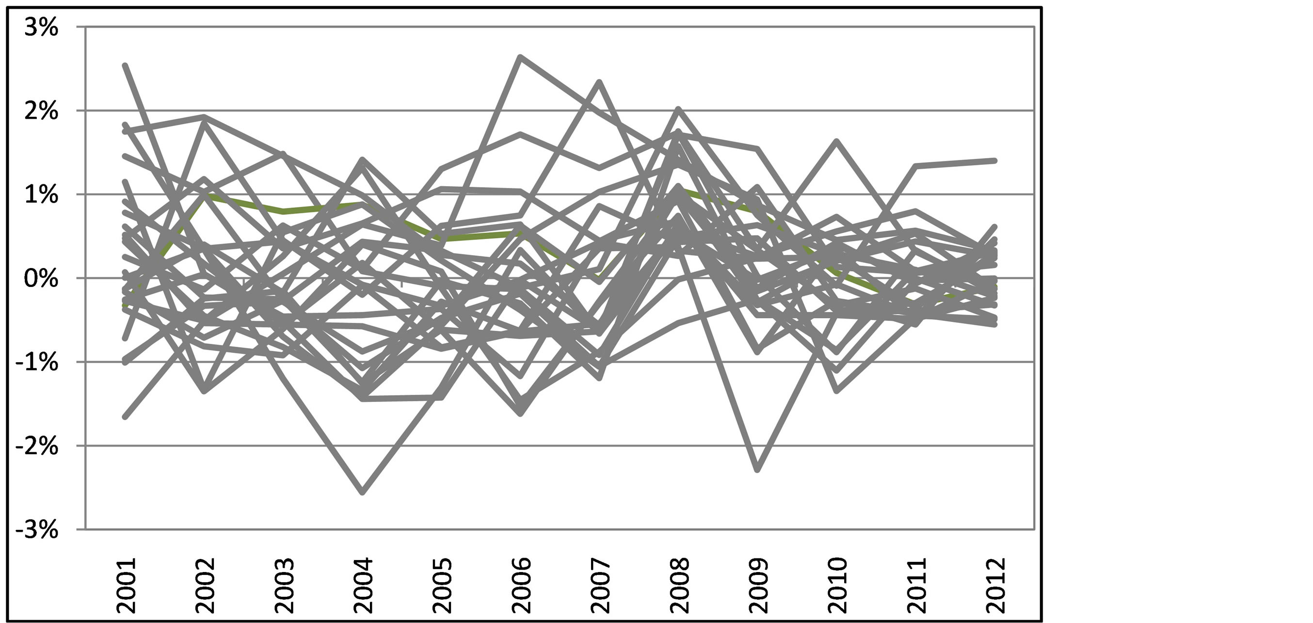
Figure 3. USA: inflation rate (%) main 25 cities and areas (National Rate = 0). Data from US Department of Labor, Bureau of Labor Statistics [15] .
The 17 countries of the European Monetary Union (EMU) (Figure 4), show a higher degree of dispersion but if we remove from the graph countries as Estonia, Slovakia and Slovenia, recent members of EMU, the rest behave similarly to Mexico and the USA, that is, within range (+/−) 2% inflation around the area average.
The problem appears when we consider not the annual inflation rate but it’s accumulated. In an optimal currency area the dispersion is reduced because inflation differentials revolve around average inflation while in a not optimal area they accumulate away from the average as we see in Figure 5 in which we compare the behavior of the EU and the USA.
In the case of EMU we should make an additional comment about inflation and is its relation to the current account balance in the balance of payments (BOP). The quantity theory of money has repeatedly taken the cash flow model developed by David Hume [16] in the second half of the eighteenth century to explain how a nationcall A-with a positive trade balance will lose it advantage through inflation caused by an increase in circulating currency. While this happens, the negative trade balance of trade partner-nation B-causes a decrease in its money

Figure 4. Euro zone: inflation rate (%) 17 countries (HICP = 0). Data from Eurostat [13] .
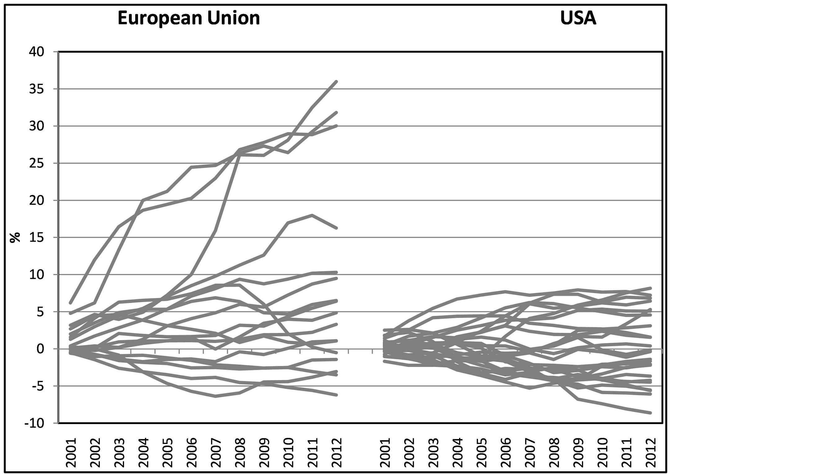
Figure 5. Euro zone: accumulated inflation (%) 17 countries (HICP = 0). Data from Eurostat [13] . And USA accumulated inflation in main cities data from US Department of Labor, Bureau of Labor Statistics [15] .
supply leading to deflation, thus regaining its market advantage by reducing the relative prices of exportable production.
Regardless of whether the model of Hume takes place under the gold standard, a trade deficit leads to an increase in the debtor part to the BOP which means higher interest rates and therefore forces that should reduce inflation. The reality is not so and the case of the nations that conform the euro zone is a clear example. Let’s see it.
From 2001 to 2012 Germany, for example, accumulated a surplus in its balance of goods and services for a total of 1,839,183 millions of Euros. In the same period the accumulated inflation in that country was 23%, the lowest in the euro zone. In the case of Spain, on the other hand, in the same period with an accumulative inflation of 39.5%—the thirteenth highest in the area-had the highest cumulative current account deficit: 738,260 millions of Euros.
Table 2 shows us the behavior of the variables identified for the 17 EMU countries. We note that from the seven countries with accumulated surplus in the trade balance of goods and services during the 12 years studied, five of them had the lowest inflation rates accumulated in the same period. The only exceptions were Austria and France.
In same table, on the other hand, we note that of the ten countries with continuous deficit in the trade balance, eight of them had the higher cumulative inflation in the region, with the exception of Slovakia and Slovenia.
It follows that financial capital movements are playing an important role in the setting according which Hume hypothesis should be reached. However, since a negative and permanent trade balance resembles a financial pyramid, at the time that the net inflow of capital halt or reverse, as is happening lately in Spain, Greece and, more recently in Cyprus, in the absence of the devaluation mechanism to adjust the real sector of the economy, the resulting recession could only be adjusted with a fall in domestic prices, including wages.
3.6. Currency Areas and Unemployment
The unemployment rate for states or regions of a country is a significant variable in order to meet the mobility of labor and financial capital, as well as the existence of central fiscal policies that allow a redistribution of national income between regions.
In order to know how the economy behaves in the micro level of a currency area, converting the national or regional rate to zero allows us to observe this variable inside the unit studied.
In Figure 6 we see the evolution of the unemployment rate of each of the 32 states of Mexico over the national average.
Table 2. Cumulative inflation (HICP) and external balance of goods and services of euro zone members 2001-2012. Source Eurostat [17] .

Figure 6. Mexico: unemployment rate (%) 32 States (National Rate = 0). Data from Instituto Nacional de Estadistica y Geografia (INEGI) [18] .
We note that the global crisis that began in 2008 caused local unemployment rates greater than the national average and that as economic growth came back, they converge again but not in the pre-crisis levels.
In Mexico state rates move today within +2% and −3% while in the pre-crisis the range was closer to (+/−) 1%.
For the US (Figure 7), the behavior is similar but shows a greater dispersion during the economic crisis.
Again, as in the case of Mexico, the States of the American Union are oscillating between +3% and −4%. We also note that unemployment levels prior to the crisis are not recovering quickly but the tendency is to approach to the national average.
The case of the Euro zone (Figure 8) is different as we observe a tendency to spread due to the high unemployment rate, currently up to 25% in Spain and Greece, and above 10% in 8 other countries in the area. This is indicative of the worsening of the economic recession in the region.
3.7. Are Inflation and Unemployment, a Dilemma?
In economic books we read that in macroeconomic policy we are faced with the dilemma of choose between unemployment and inflation. Data from Europe seem to show that no such dilemma exists; on the contrary, inflation and unemployment move together. Some may think that we are faced with the phenomenon of stagflation economic stagnation with inflation—but it is not, what we see is growing recession with inflation, although in the last year we are observing a drop over previous levels, but still above the area average.
What follows are two graphs in which we observe the behavior, since the crisis began in 2008, of the accumulated inflation and the unemployment rate in two of the hardest-hit countries in the Euro zone: Spain and Greece. In the case of Spain (Figure 9), the degree of correlation between the two variables is 0.8418.
In Greece (Figure 10) the correlation among the variables unemployment and cumulative inflation is even bigger: 0.9383. Both are moving together in the same direction and none of them is the independent variable.
4. Conclusions
In our analysis, the euro crisis has led us to interesting issues of theory and economic policy. It has shown us, without a doubt, that the European Monetary Union is not an optimal currency area and has given the reason to several thinkers based on the initial contributions of Robert A. Mundell which have provided evidence that allowed us to see that the theory of free trade zones was wrong in holding that the monetary union could be achieved before the political union. Today we realize that the euro crisis is due to the absence of shared monetary and fiscal policies, to the lack of a central bank that fulfills its role as a lender of last resort, as well as a banking union that still sees far, according to recent statements made by Stanley Fischer.
According to my analysis, we should include as currency areas and individual countries, not only the euro zone but also other areas where there are prevailing currencies as Dollar, Euro, Sterling pound, etc. This allows us

Figure 7. USA: unemployment rate (%) 50 States, plus DC and puerto rico (National Rate = 0). Data from US Department of Labor, Bureau of Labor Statistics [19] .
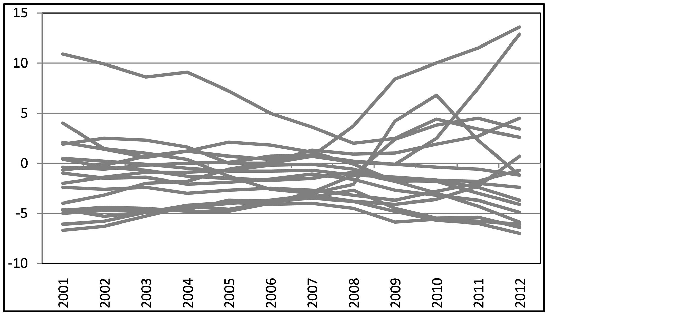
Figure 8. Euro zone: unemployment rate (%) 17 countries (Euro Zone = 0). Data from Eurostat [20] .
to make valuable comparisons.
I consider that it was a mistake of the way that the Treaty of Maastricht established inflation requirements to countries in the euro area. It is wrong to talk about annual rates instead of accumulated rates. We note that in countries like USA and Mexico, the divergence from the national average inflation remains within narrow margins while several EMU countries moved constantly away from the average of the zone with the consequent loss of trade competitiveness.
The global financial structure allows countries with positive current account balances to have lower inflation rates than those who have accumulated large trade deficits. These positive balances are provided to countries that have negative balances, thus financing their imports.
The relative free mobility of labor in countries like USA and Mexico makes local unemployment rates oscillate in a narrow range of +/− 3% or 4%. Countries in the euro area have shown ample variations ranging from +14% to −7%.
To apply austerity policies instead of expanding the money supply has led inflation and unemployment to

Figure 9. Spain, cumulative inflation rate and unemployment rate (%). Eurostat [21] .

Figure 10. Greece, cumulative inflation rate and unemployment rate (%). Eurostat [21] .
move in the same direction. In recent years, countries such as Greece, Spain, Ireland and Portugal, among others, have suffered something worse, recession with inflation rather than facing the dreaded stagflation-stagnation with inflation.
References
- Mundell, R.A. (1961) A Theory of Optimum Currency Areas. The American Economic Review, 51, 509-517.
- Encinas Ferrer, C. (2009) Análisis de la balanza de pagos bajo dolarización. Hacia una teoría de las áreas monetarias no óptimas. (Analysis of Balance of Payments under Dollarization. Towards a Theory of Nonoptimal Currency Area. Principios, Estudios de Economía Política, 2009. http://www.sistemadigital.es/media/PDF/PPios15_carlos%20encinas.pdf
- Samuelson, P.A. and Nordhaus, W.D. (2010) Macroeconomia, con aplicaciones a America Latina. Mc Graw Hill, Mexico, 313.
- McKinnon, R.I. (1963) Optimum Currency Areas. The American Economic Review, 53, 717-725. http://www.experimentalforschung.vwl.uni-muenchen.de/studium/veranstaltungsarchiv/sq2/mckinnon_aer1963.pdf
- Krugman, P. (2013) The Triumph of Peter Kenen, the Revenge of Robert Mundell. The Conscience of a Liberal, the New York Times. http://krugman.blogs.nytimes.com/2013/06/03/the-triumph-of-peter-kenen-the-revenge-of-robert-mundell/
- Kenen, P. (1969) The Theory of Optimum Currency Areas: An Eclectic View. In: Mundell, R. and Swoboda, A., Eds., Monetary Problems of the International Economy, The University of Chicago Press, Chicago.
- Tugores Ques, J. (2013) La crisis europea: Lecciones e implicaciones. Conference at Coloquio Internacional La Crisis del euro y su Implicaciones Económicas y Sociales, Universidad De La Salle Bajío, 29-30 August 2013.
- Reinhart, C.M. and Rogoff, K.S. (2010) Growth in a Time of Debt. American Economic Review, American Economic Association, 100, 573-578.
- Reinhart, C.M. and Rogoff, K.S. (2013) Reinhart-Rogoff Response to Critique. The Wall Street Journal. http://blogs.wsj.com/economics/2013/04/16/reinhart-rogoff-response-to-critique/
- Krugman, P. (2013) Reinhart-Rogoff, Continued. In: The New York Times, the Conscience of a Liberal. http://krugman.blogs.nytimes.com/2013/04/16/reinhart-rogoff-continued/
- Watt, A. (2013) A Brief Social Science Methodology Primer—Renowned Harvard Economists Please Take Note. Social Europe Journal. http://www.social-europe.eu/2013/04/a-brief-social-science-methodology-primer-renowned-harvard-economists-please-take-note/
- Herndon, T., Ash, M. and Pollin, R. (2013) Does High Public Debt Consistently Stifle Economic Growth? A Critique of Reinhart and Rogoff. http://www.peri.umass.edu/fileadmin/pdf/working_papers/working_papers_301-350/WP322.pdf
- European Commission, Eurostat (2013) Statistics Database, International Trade. http://epp.eurostat.ec.europa.eu/portal/page/portal/statistics/search_database
- Instituto Nacional de Estadística y Geografía, INEGI (2013) Banco de Información Académica, Precios e Inflación, Indice Nacional de Precios al Consumidor. http://www.inegi.org.mx/sistemas/bie/
- US Department of Labor, Bureau of Labor Statistics (2013) http://data.bls.gov/pdq/SurveyOutputServlet
- Hume, D. (1752) Political Discourses. London. http://www.davidhume.org/texts/pd.html
- European Commission, Eurostat, Statistics Database, International Trade (2013) Population and Social Conditions, Employment and Unemployment. http://epp.eurostat.ec.europa.eu/portal/page/portal/statistics/search_database
- Instituto Nacional de Estadística y Geografía, INEGI (2013) Banco de Información Académica, Tasa de ocupación, desocupación, subocupación (Resultados mensuales del ENOE), Tasa de desocupación por entidad federativa como promedio móvil de tres con extremo superior. http://www.inegi.org.mx/sistemas/bie/
- US Department of Labor, Bureau of Labor Statistics (2013) Local Area Unemployment Statistics. http://data.bls.gov/cgi-bin/surveymost?la
- European Commission, Eurostat (2013) Statistics Database, International Trade. Population and Social Conditions, Employment and Unemployment. http://epp.eurostat.ec.europa.eu/portal/page/portal/statistics/search_database
NOTES

1In the recent International Monetary Fund Fourteenth Jacques Polak Annual Research Conference, held November 7 and 8, 2013, Stanley Fischer considered that the Banking Union was in the future but when asked about dates of that future he said that it will take a very long term.
2Hamilton, Alexander quoted by the Bureau of the Public Debt, United States Department of the Treasury. http://www.publicdebt.treas.gov/

3A budget deficit of 3% becomes a debt greater than 60% of GDP in just 17 years and that’s assuming that we started from a zero level, which did not occur in any of the original countries of EMU or were subsequently admitted.