Theoretical Economics Letters
Vol.4 No.7(2014), Article ID:48483,10 pages
DOI:10.4236/tel.2014.47070
A Model of Manufacturers and Buyers of Cars over the Business Cycle Illustrating Competitive Manufacturing
Gerald Aranoff
Ariel University Center of Samaria, Bnei Brak, Israel
Email: garanoff@netvision.net.il
Copyright © 2014 by author and Scientific Research Publishing Inc.
This work is licensed under the Creative Commons Attribution International License (CC BY).
http://creativecommons.org/licenses/by/4.0/


Received 2 June 2014; revised 1 July 2014; accepted 1 August 2014
ABSTRACT
We illustrate competitive manufacturing with an original theoretical model of manufacturers and buyers of cars over a business cycle that have peak and off-peak demand periods. There are two types of plants manufacturing cars, plantK and plantL, each having linear total costs with absolute capacity limits. PlantK operates with low VC and high FC by being capital intensive. PlantK is output-rates rigid since it produces throughout the business cycle and always at capacity. PlantL operates with low FC and high VC by relying on outsourcing major components and parts. PlantL is output-rates flexible since it produces only in the peak-demand periods. We show results under SRMC pricing. Then we examine an alternate arrangement which increases demand irregularity. We show, under conditions of the model, that the added cost to supply irregular demand should be small because of the low FC of plantL. We show, under the conditions of the model, that the added gain in consumer surplus to have irregular demand supplied should be large because consumers will have more available for the peak periods. The main policy implication of this theoretical model—for regularly recurring cycles—is to urge focus, even in the off-peak periods, on adequate capacity for the peak periods.
Keywords:Manufacturing, Competition, Business Cycle, Marginal-Cost Pricing, Output-Rate Flexibility

1. John M. Clark: The Economics of Overhead Costs
John M. Clark (1884-1963) wrote of the desirability of manufacturing plants to operate at their normal capacity with production costs per unit output the lowest. John M. Clark attributed the main problems of the business cycle to the dominant role of fixed costs that are incurred irrespective of output rates:
“It is needless to point out that overhead costs play a fundamental part in the behavior of business at every stage of that many-sided phenomenon, the business cycle. The part they play is most paradoxical. For they make regular operation peculiarly desirable and peculiarly profitable, so that business feels a definite loss whenever output falls below normal capacity, yet it is largely due to this very fact of large fixed capital that business breads these calamities for itself, out of the laws of its own being. And the largest businesses, which have the highest percent of constant costs due to invested capital, are, as we have seen, precisely the ones which fluctuate the most, so far as employment is an index. There is something about the commercial-industrial system which bewitches business so that it does just the thing it is trying to avoid, and is held back from doing just the thing it yearns to do—maintain steady operation and avoid idle overhead. And while the contributing causes of this strange auto-hypnosis are many and of varied character, technical, financial, commercial, and psychological; the underlying fact of large capital plays a central part, and the inelasticity of cost, sunk cost, and the shifting and conversion of overhead cost are all facts of major importance.”1 The US manufacturing industries are now some 6 or 7 years in a recession, as the figures in Table 1 show2.
In his 1923 book John M. Clark illustrated the calculations for expected average
cost,
 , for a manufacturing plant making a car3.
See Table2 The
, for a manufacturing plant making a car3.
See Table2 The
 of the car
 versus the
 . A price of $1301
per car would give zero economic profits only if %CU rates actual equalled expected.
For lower %CU, as in Table 1, a price of $1301
would give losses to car producers with losses rising as %CU falls. Clark argued
for efforts to keep %CU high as the key to efficiency and economic wellbeing.
. A price of $1301
per car would give zero economic profits only if %CU rates actual equalled expected.
For lower %CU, as in Table 1, a price of $1301
would give losses to car producers with losses rising as %CU falls. Clark argued
for efforts to keep %CU high as the key to efficiency and economic wellbeing.
2. Traditional Manufacturing versus High-Value Manufacturing
In traditional manufacturing the focus is on the production phase of a product. In high-value manufacturing the recommendation is for manufacturers to concern themselves with the entire manufacturing value chain:
“A New Definition of High-Value Manufacturing... A successful manufacturing industry goes beyond production, it means thriving research and development (R&D), design, supply management, sales and marketing as well as after sales services... Highly successful manufacturers do not need to rely on production alone and they can accommodate effective outsourcing.”4 Outsourcing means buying components and parts instead of making them. In high-value manufacturing firms

Table 1 . % capacity utilization manufacturing USA.
Table 2. Annual budgets at various operating rates.
are increasing product flexibility, meaning which products they make. In traditional manufacturing, as here and in John M. Clark’s writings, the industry is composed of manufacturers that produce a particular product, such as a car. In high-value manufacturing firms are part of other industries depending on what products they sell. In traditional manufacturing, outsourcing increases a firm’s output-rate flexibility of production of a particular product.
3. An Original Model of Manufacturing and Buying Cars over the Business Cycle
We illustrate an original model of manufacturing and buying cars over the business cycle. The product is homogeneous in that all cars are assumed identical in looks, driveability and value in the market. We assume fluctuating demand over a business cycle of a number of years, with peak periods, part of the cycle, and off-peak periods, the balance of the cycle. We assume car manufacturers set two prices, one at the peak and one for the off-peak times of the business cycle. We assume no price collusion among car manufacturers. We assume car manufacturers know the consumer-demand schedules for their cars produced. We assume zero expected profits for all car manufacturers in long-run equilibrium. Initially we assume SRMC pricing.
4. Car Manufacturing over the Business Cycle: The Supply Side
We assume a single homogeneous product, Q, cars. We assume ease of entry of new
car manufacturers. We assume a business cycle of two states of demand,
 and
and , off-peak and peak, each with
a likelihood, where the likelihoods add to one. There are two types of car manufacturing
plants, plantK and plantL. Car manufacturing plants require
durable and specific assets, and have linear short-run total-cost curves with absolute
capacity limits. Car manufacturing plants have a per-car variable-operating cost
, off-peak and peak, each with
a likelihood, where the likelihoods add to one. There are two types of car manufacturing
plants, plantK and plantL. Car manufacturing plants require
durable and specific assets, and have linear short-run total-cost curves with absolute
capacity limits. Car manufacturing plants have a per-car variable-operating cost , per-car capacity costs
 (fixed costs per-year per-plant divided by maximum cars production rate per-year
per-plant) and per-plant capacity
(fixed costs per-year per-plant divided by maximum cars production rate per-year
per-plant) and per-plant capacity
 (maximum cars production per-year per-plant).
We envision investors and managers walking into a car manufacturing plant store
that has two shelves: each with a model plant
 that costs, say, $1,000,000 to build. On one shelf is a model of plantK
and on the other shelf is a model plantL (see
Figure 1). Investors or entrepreneurs can order any multiple or fraction
of the model plants. No economies of scale exist for plants. Thus the long-run marginal
cost (LRMC) and long-run average cost (LRAC) for plants in the car manufacturing
plant store are horizontal. These customers of the car manufacturing plant store
have to decide plantK and choose a
that costs, say, $1,000,000 to build. On one shelf is a model of plantK
and on the other shelf is a model plantL (see
Figure 1). Investors or entrepreneurs can order any multiple or fraction
of the model plants. No economies of scale exist for plants. Thus the long-run marginal
cost (LRMC) and long-run average cost (LRAC) for plants in the car manufacturing
plant store are horizontal. These customers of the car manufacturing plant store
have to decide plantK and choose a
 or plantL and choose a
 . The assets are durable
and specific meaning that the plants will last a long time, say 50 years, and are
useful only for making cars.
. The assets are durable
and specific meaning that the plants will last a long time, say 50 years, and are
useful only for making cars.

Figure 1. SR total-cost curves of plantK and plantL.
4.1. Key Assumptions
The key assumptions of the model are:
A1: ,
,
 , and
, and
 as in Figure 2. The curves in
Figure 2 must cross or else the lower one will dominate.
as in Figure 2. The curves in
Figure 2 must cross or else the lower one will dominate.
A2: Demand fluctuates with frequencies,
 in off-peak and
 in peak and
 .
.
A3: We assume SRMC (short-run marginal-cost) pricing behavior. With linear TC functions and SRMC pricing, plants will operate at either 0% or 100%.
A4: We assume market prices in off-peak times :
:
 and market prices in peak times
 :
: . Thus plantsK operate
at capacity at all times, while plantsL shutdown in
. Thus plantsK operate
at capacity at all times, while plantsL shutdown in
 and operate at capacity in
 . Total cars manufactured
and sold in the industry in the off-peak period is
. Total cars manufactured
and sold in the industry in the off-peak period is
 where
where . Total car manufactured and sold in the industry
in the peak period is
. Total car manufactured and sold in the industry
in the peak period is
 where
where .
.
A5: Long-run equilibrium requires zero expected profits for both plant types.
4.2. Objective of Proposition 1
We prove in the following proposition the conditions of indifference for investors to choose between plantK and plantL in LR equilibrium.
4.3. Proposition I
Proposition 1 Under Assumptions A1 through A5 with both plants used in long-run equilibrium, then it must be true:
 (1)
(1)
If
 (that is, the left-side inequality is violated) then only plantL will
be used. If
(that is, the left-side inequality is violated) then only plantL will
be used. If
 (that is, the right-side inequality is violated) then only plantK will
be used.
(that is, the right-side inequality is violated) then only plantK will
be used.
Proof: Investors in plantK have zero expected economic profits per Assumption A5:
 (2)
(2)
This gives us:
 (3)
(3)
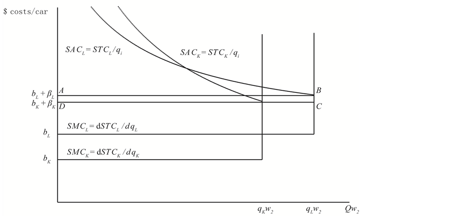
Figure 2. PlantL
added cost of supplying irregular demand: .
.
Investors in plantL have zero expected economic profits per Assumption A5:
 (4)
(4)
This gives us:
 (5)
(5)
Equations (3) and (5) can be combined:
 (6)
(6)
For plantsL to shut-down in the off-peak period per Assumption A4 must
be . If
. If
 then, strictly speaking, plantsL are indifferent to operating and some
may be operating. Using Equation (6), this requires:
then, strictly speaking, plantsL are indifferent to operating and some
may be operating. Using Equation (6), this requires:
 (7)
(7)
Since , We can write:
 (8)
(8)
which is the asserted left-side inequality condition:
 (9)
(9)
By Assumption A4,
 , plantsK earn a positive contribution
margin in
, plantsK earn a positive contribution
margin in . If
. If
 then plantsK, would shut-down in
 .
.
By Assumption A4,
 , plantsL earn a positive contribution
margin in
, plantsL earn a positive contribution
margin in . If
. If
 then plantsL, would shut-down in
 .
.
 give zero profits to plantsK with
 . Profits are zero
because in
. Profits are zero
because in
 plantsK earn no contribution margin. In
 plantsK earn contribution margin
 or
or
 which exactly equals their fixed costs. With
 for equilibrium and zero economic profits

Thus
 (10)
(10)
yields the right-side inequality condition assertion.
4.4. Left-Side and Right-Side Inequality Conditions
The left-side condition in (1) is that . If one more car is supplied
in both peak and off-peak times, the total cost over the cycle of a 1 car capacity
plant operated over the cycle is
. If one more car is supplied
in both peak and off-peak times, the total cost over the cycle of a 1 car capacity
plant operated over the cycle is
 since
since . A price of
 in both time periods will exactly cover costs of one extra car operating in both
periods. We suggest calling this condition that plantK be more static
efficient, in the sense of Clark’s use of the term static in that there are no business
cycles [2] 5.
in both time periods will exactly cover costs of one extra car operating in both
periods. We suggest calling this condition that plantK be more static
efficient, in the sense of Clark’s use of the term static in that there are no business
cycles [2] 5.
The right-side condition in (1) is that . Assume we need one more
car over the cycle only to meet peak demand. A price of
. Assume we need one more
car over the cycle only to meet peak demand. A price of
 will exactly cover costs of one extra car over the cycle manufactured only in high-demand.
The right-hand condition is that where production is used only in high-demand times, plantL is superior. The right-hand condition requires that SACL be flatter shaped than SACK. We define output flexibility as the relative flatness of the SAC curve. We suggest calling this condition that plantlL be more output-rates flexible efficient6.
4.5. PlantL Added Cost of Supplying Irregular Demand:

If demand for cars were static with no irregularities, then firms would choose only
plantK and . Demand for cars is irregular
in the model, fluctuating between
. Demand for cars is irregular
in the model, fluctuating between
 and
and . The added cost of supplying irregular demand in
the model is borne entirely by plantL where
. The added cost of supplying irregular demand in
the model is borne entirely by plantL where .
.
Thus, a measure of added cost of supplying irregular demand in the model would be
the expected manufactured cars to meet peak demand × the difference in SRAC
between the two plants, or: . See
Figure 2 which shows the added cost of supplying irregular demand for
a single plantL (rectangle
. See
Figure 2 which shows the added cost of supplying irregular demand for
a single plantL (rectangle ).
).
5. Cars over the Business Cycle: The Demand Side
5.1. Definition of the Model and Its Terms and Assumptions
There are two groups in our hypothetical society: Suppliers (manufacturers of cars) and consumers (households who buy cars). Consumers buy cars in a free market on a daily basis from various manufacturers where each manufacturer posts its prices. Consumers pay the lowest price per-car in the local market. The intersection of this price with the consumer-demand schedules (off-peak and peak) determine the quantity of cars the consumers order.
Consumers have a fixed budget for car purchase expenditures. They are price sensitive
in buying cars, in the sense that consumers will buy more cars at a lower market
price and less cars at a higher market price. Consumers pay market price times quantities
purchased,
 (total revenue to suppliers equals market price times quantities).
The demand curve shows the maximum quantities consumers would be willing to purchase at various prices. The assumption is that the demand curve is downward sloping, meaning that consumers would be willing to buy more cars if prices were lower, all else being the same. The area under the demand curve up to the point of quantities of market purchases shows the value to the consumer.
Figure 3 shows a geometric demonstration with varying
pricing (alternative A) versus fixed pricing (alternative B) with fluctuating D
functions, off-peak period and peak period each with its associated . Let
. Let
 be consumer demand for cars during off-peak periods, the great majority of the year,
say 6/7th of the year.
be consumer demand for cars during off-peak periods, the great majority of the year,
say 6/7th of the year.
Using hypothetical numbers to make the economic concepts clearer, point K could be that, at a market price of $36 per car consumers are willing to buy 35 cars. Point H might be that at a market price of $33 per car consumers are willing to buy 37 cars.
Let
 be consumer demand for cars on the peak period. Using hypothetical numbers to illustrate,
point D could be that, at a market price of $51.9 per car consumers are willing
to buy 42 cars. Point J could be that, at a market price of $36 per car consumers
are willing to buy 54 cars per day.
be consumer demand for cars on the peak period. Using hypothetical numbers to illustrate,
point D could be that, at a market price of $51.9 per car consumers are willing
to buy 42 cars. Point J could be that, at a market price of $36 per car consumers
are willing to buy 54 cars per day.
The demand curve , off-peak period demand,
occurs with frequency,
, off-peak period demand,
occurs with frequency,
 , 6/7. The demand curve
 . Peak period demand, occurs
with frequency,
. Peak period demand, occurs
with frequency,
 , 1/7.
We define consumer surplus as the area under the demand curve and above the price
line. We define expected values, E, as the sum of each outcome times its expected
value. Using the illustrated numbers for points H and D, the market equilibrium
points for pricing rule A, varying prices, we can calculate , expected total revenue,
and
, expected total revenue,
and , expected quantities, as follows:


Using the illustrated numbers for points K and J, the market equilibrium points
for pricing rule B, fixed prices, we can calculate , expected total revenue,
and
, expected total revenue,
and , expected quantities, as follows:


5.2. Objective of Proposition II
We prove in the following proposition that consumer surplus is necessarily larger in an arrangement where consumers get more cars for the peak period at the cost of less cars for the off-peak periods whereby consumers pay
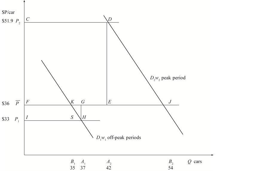
Figure 3.
 Pricing adds consumer surplus:
 .
.
the same amount and buy the same number of cars over the year. We show graphically this increase in consumer surplus. This becomes a maximum willingness for consumers to pay suppliers for that arrangement.
We assume that suppliers are willing to offer cars according to two alternative
pricing schemes: a fixed price,
 , at all times, versus
 for off-peak periods and
 for the peak period. We have two basic assumptions in the model: according to both
pricing schemes total payments over the week are the same and total quantities purchases
are the same.
for the peak period. We have two basic assumptions in the model: according to both
pricing schemes total payments over the week are the same and total quantities purchases
are the same.
5.3. Proposition II
Proposition 2 A comparison of alternative pricing schemes, A: varying prices, versus
B: fixed prices, under conditions of shifting downward-sloping demand curves shows
 and rises as demand elasticity rises assuming
 (11)
(11)
and
 (12)
(12)
Proof: By definition of :
:
 (13)
(13)
and
 (14)
(14)
By definition of :
:
 (15)
(15)
and
 (16)
(16)
By definition of :
:
 (17)
(17)
and
 (18)
(18)
By Assumption (11) We can state:
 (19)
(19)
By Assumption (12) We can state:
 (20)
(20)
Combining Assumptions (11) and (12):
 (21)
(21)
Rearranging:
 (22)
(22)
Using the letters of the Figure 3:
 (23)
(23)
This is important because it shows consumer-surplus comparisons for perfectly inelastic,
zero price elasticity,
 and
and , meaning that consumers demand
 in
in
 and
and
 in
in
 for all prices.
We can state:
 (24)
(24)
Rearranging:
 (25)
(25)
We can state:
 (26)
(26)
Using the results of Equation (23), We can state:
 (27)
(27)
Thus,
 must be greater than zero, providing that price
elasticities of the demand curves are not zero. At zero price elasticity
must be greater than zero, providing that price
elasticities of the demand curves are not zero. At zero price elasticity
 and
and
 and therefore areas
 and
and
 each equals zero.
 rises as price elasticity rises, since the areas
of
rises as price elasticity rises, since the areas
of
 increase with more elastic demand curves.
5.4.
 Pricing Adds Consumer Surplus:

 represents the gain in consumer surplus with fixed
pricing over varying pricing that gives the same expected TR to suppliers and same
expected Q to consumers. Theoretically
represents the gain in consumer surplus with fixed
pricing over varying pricing that gives the same expected TR to suppliers and same
expected Q to consumers. Theoretically
 is a maximum willingness to pay for an arrangement of an increase in irregularity.
This is a beginning of constructing a demand schedule for irregularity. The increase
in irregularity is going from
is a maximum willingness to pay for an arrangement of an increase in irregularity.
This is a beginning of constructing a demand schedule for irregularity. The increase
in irregularity is going from
 to
to . We could test maximum willingness to pay to increase
irregularity further or for a lesser degree of increase irregularity. We could explore
the effects on consumer surplus with alternative pricing schemes that expected payments
rise or expected Q falls.
. We could test maximum willingness to pay to increase
irregularity further or for a lesser degree of increase irregularity. We could explore
the effects on consumer surplus with alternative pricing schemes that expected payments
rise or expected Q falls.
6. Future Research Questions and Policy Implications
We present here an original theoretical model of manufacturers and buyers of cars over a business cycle that have peak and off-peak demand periods to illustrate competitive manufacturing. We permit two types of car manufacturing plants, plantK operated year around and plantL opens only in peak-demand times. PlantK is static efficient but output-rates rigid while plantL is output-rates flexible but static inefficient. These are the two conditions for co-existence of diverse plant types.
To make policy recommendations, we need research on how realistic and critical are the assumptions of the model. Areas of future research include relaxing the assumption of linear total costs with absolute capacity limits. The more firms can produce beyond their normal capacity such as by paying over-time reduces the need for plantL.
The model here assumes easy entry which should eliminate super-normal profits over time. The ease of entry of the model for car manufacturing may be realistic today with the vast increase in outsourcing and in world trade. With internet, computers and smart-phones, firms could rely on suppliers to make parts and components and deliver them “just-in-time”. This is plantL of the model—a factory that is largely assembly only. The model assumes parts and factor-input prices remain constant. If they rise with shifts to plantL this would lessen the advantages of plantL.
What may be surprising is that in the model of the paper consumers have a huge willingness
to pay to get suppliers to switch from SRMC pricing to a fixed-year around price
(triangles
 in Figure 3) with the cost to provide for accentuated
fluctuations small (rectangle
in Figure 3) with the cost to provide for accentuated
fluctuations small (rectangle
 in Figure 2).
Consumers have a huge willingness to pay, in the model of the paper, for the car manufacturers to switch from SRMC pricing, because the consumers will be buying more cars in the peak of the business cycle, when their demand is high. Making the peak of the business cycle better, adds considerably to consumer welfare even though the peak is infrequent. The gains to consumers increase with more price elasticity of demand curves. Making the cost of a car higher in the off-peak is less importance, though the off-peak is far more frequent. Likely that consumer demand curves are elastic in high-demand times more so than in low-demand times, especially for cars. This would further increase the importance of focusing on sufficiency of supply for the highdemand periods.
The policy implication of this theoretical model is that though capacity utilization rates today are low as we’re in the off-peak period of the business cycle, we advise investors to think of the peak period and to plan for it. Investors should invest in plantL today. They will be amply rewarded during the peak of the business cycle with only a modest investment today7.
This is an important lesson—for regularly recurring cycles—because it urges focus, even in the off-peak periods, on making the peak periods better. This agrees with business cycle theories that urge social focus on increasing and prolonging cyclical peaks. This supports John M. Clark’s workable competition thesis [3] . John M. Clark was on the side of big businesses and so-called monopolies and cartels8. Clark argued that new entry (even the threat of it) will keep monopolies and cartels sufficiently competitive to be workably competitive. Clark defended the US cement industry’s basing point price system which the US courts outlawed.
References
- Clark, J.M. (1923) Studies in the Economics of Overhead Costs. The University of Chicago Press, Chicago.
- KPMG (2012) A Comprehensive View of Australian manufacturing. November 2012, kpmg.com.au.
- Aranoff, G. (2011) Competitive Manufacturing with Fluctuating Demand and Diverse Technology: Mathematical Proofs and Illuminations on Industry Output-Flexibility. Economic Modelling, 28, 1441-1450. http://dx.doi.org/10.1016/j.econmod.2011.02.016
- Aranoff, G. (1991) John M. Clark’s Concept of Too Strong Competition and a Possible Case: The US Cement Industry. Eastern Economic Journal, 17, 45-60.
NOTES

1John M. Clark, page 386 .
2Source: www.federalreserve.gov
3John M. Clark, page 185 .
4KPMG, pages 8-9 . Outsourcing is a modern term. John M. Clark notes that where a single integrated firm produces an intermediate and a final product, the result is a higher proportion of fixed costs, e.g. “When a concern buys materials, the constant part of the cost of producing them becomes a variable cost to the user; if the maker and user were integrated, the combination would show a larger proportion of constant costs than do the two concerns separately.” “Overhead Costs,” by John M. Clark Encyclopedia of the Social Sciences 1933, volume 9 page 512.

5For example, John M. Clark page 465: “In a perfect static state where there were no business cycles nor other unpredictable irregularities, supply would come much nearer to equality with demand ...”
6See Gerald Aranoff and references cited .

7An real-world example of plantL that requires only a modest investment is the Reuters July 2014 item “In Ghana, a novel way to test the consumer market: micro factories let companies jump into countries to gauge demand without major investment.”
8See, “Monopoly” by John M. Clark, Encyclopedia of the Social Sciences, 1933, volume 10 623-629.