Journal of Mathematical Finance
Vol.05 No.04(2015), Article ID:61461,8 pages
10.4236/jmf.2015.54033
Predictive Analytics on CSI 300 Index Based on ARIMA and RBF-ANN Combined Model
Lyuxun Yang, Xi Cheng
The School of Statistics and Mathematics, Zhongnan University of Economics and Law, Wuhan, China

Copyright © 2015 by authors and Scientific Research Publishing Inc.
This work is licensed under the Creative Commons Attribution International License (CC BY).


Received 20 October 2015; accepted 22 November 2015; published 25 November 2015

ABSTRACT
The time series of share prices is a highly noised, non-stationary chaotic system which possesses both linear and non-linear characteristics. The alternative of either linear or non-linear prediction models is of its inherent limitation. The paper establishes an ARIMA and RBF-ANN combined model and makes a short-term prediction on the time series of CSI 300 index by choosing various typical input variables. Results show that the combined model with multiple input indicators, compared with single ARIMA model, single RBF-ANN model, or models with single input variable, is of higher precision.
Keywords:
ARIMA, RBF-ANN, CSI 300 Index, Prediction Model

1. Introduction
Prediction model of share price or index is of both practical and theoretical significance. Y. Bai [1] has made a forecast on Shanghai securities composite index by using ARIMA model. J. Ouyang [2] and X. Yang [3] have made a forecast on the rise and fall of share prices by using different improved methods of BP neural network models, which has made some effects. However, share price is influenced by complicated factors such as economy, politics and society. Its mathematic model is a highly noised, non-stationary chaotic system [4] with both linear and non-linear characteristics. So, to individually make predictions with linear and non-linear models has some certain limitation. In addition, since the change of share price or index is related to lots of factors, it is not proper to only select historical value sequence as the input variable.
Autoregressive Integrated Moving Average (ARIMA) Model is a notable model in time series data prediction [5] and is widely used in econometrics study. It fits the linear characteristics of non-stationary time series to some extent. With a good ability of functional approximation, Artificial Neural Network (ANN) can explore the non-linear law of time series to a large extent. However, the conventional Back Propagation (BP) neural network has many defects, such as difficulty in determining hidden layer unit numbers, slowing rate of convergence and tendency to local minimum. Its modeling process can even be called “the process of artistic creation” [6] . The neural network of Radial Basis Function (RBF) can effectively improve the above-mentioned defects and has been successfully used in different fields such as none-linear functional approximation, data classification and picture processing with its fast learning and good fitting sufficiency. This paper proposes a method to combine the ARIMA model with RBF neural network model, which makes full use of the characteristics of both to predict linear and non-linear rules so as to select various indicators such as the stock price index, its amplitude and transaction volume as the combined input variables of the neural network, thus promoting the preciseness of index prediction models.
2. Establishment of Prediction Models
2.1. ARIMA Model
ARIMA model is to turn integrated time series into stationary time series, and then recovering its lagged value of dependent variables, present values and lagged values of stochastic error terms.
If the sequence  can be turned into steady sequence
  via d-order difference, to introduce the delay operator B, namely:
 . (1)
. (1)
We can establish ARMA (p, q) Model, which is:
 . (2)
. (2)
In this Equation,  is the stochastic error term. After introducing the delay operator B, ARMA (p, q) Model can be expressed as:
 . (3)
. (3)
From the view of operation, the ARIMA modeling idea of Box and Jenkins can be summarized into 6 steps:
1) To carry out a stationary test on the sequences (such as the ADF unit root test). When the sequences fail to meet the condition of smoothness, turn the sequence into stationary sequences via differential transform (or logarithm differential transform);
2) To determine the order of ARIMA model by generally using Auto Correlation Function (ACF) and Partial Auto Correlation Function (PACF) for preliminary order determination, as well as Akaike Information Criterion (AIC) and Schwarz Criterion (SC) for quantization order determination;
3) To estimate the model parameters and test the significance of parameters so as to evaluate their rationality and adjust the model;
4) To carry out hypothesis test so as to check whether the diagnosis of the residual sequence is white noise. However, for the combined model illustrated below, since the residual of ARIMA model shall be fitted by other models, it shall still work when this hypothesis test is not passed;
5) To carry out diagnostic analysis so as to confirm that the obtained model is in accordance with the observed data characteristics;
6) To use the adopted model to predict the analysis.
2.2. RBF Neural Network Model
2.2.1. RBF Neural Network Structure
RBF Neural Network is a novel, effective feed forward artificial neural network with faster learning convergence rate. Theories show that RBF Neural Network can approximate any continuous rational function and possess the Best Approximation ability which the BP neural network doesn’t possess [7] [8] . The RBF Neural Network structure includes the input layer, hidden layer and output layer. As is shown in Figure 1, the input layer maps the input signals to the hidden space. The hidden layer has several hidden unit nodes and carries out non-linear mapping on input vectors via mapping function RBF. The output layer applies the mapping mode of

Figure 1. RBF neural network structure.
linear weighting to the output signals of the hidden layer.
RBF is usually defined as a monotone function of Euclidean distance between two random points in space. It is a non-negative, non-linear function with radial symmetry and bi-directional attenuation. The most common is Gaussian Function:
 (4)
(4)
In the Equation,  is the i-th input sample.
  are respectively the center and variance of the j-th node in the hidden layer.
  are respectively the amount of nodes in the input and hidden layers.
  is Euclidean norm. Now, the linear function of the output layer is:
 . (5)
. (5)
In the Equation,  is the k-th output signal.
  is the hyperlink weight from the j-th node in the hidden layer to the k-th output in the k-th output layer.
  is Gaussian Function.
2.2.2. The Learning Process of RBF Neural Network
The learning process of RBF Neural Network can be classified into unsupervised and supervised learning. The unsupervised learning process is used to learn how to solve the center and variance of a primary function. The common K-means clustering algorithm is to cluster training samples and solve center of clustering , then solve the variance via the following Equation:
 . (6)
. (6)
In the Equation:  is the maximum range from the j-th data center to any other one. n is the amount of the nodes in the hidden layer.
Supervision of the learning stage aims to determine the link weight . The least square method of repeated iteration is mainly used, namely to continuously calculate the output values and compare the calculated value with the actual value and to adjust the relevant
  according to the OLS principle while carrying out repeated correction until the output error of mean square has reached the required preciseness. After it’s done, all the parameters can be determined, namely to be used to predict the unknown output value of some group of known input volume.
2.3. Combined Model of ARIMA and RBF-ANN
The time series  of share price can be divided into three parts:
 (7)
(7)
 is a linear part to meet the conditions of autoregressive integration and moving average rules, which can be predicted with ARIMA model;
  is a predictable part in the non-linear part which doesn’t meet the general regularity but can be predicted with RBF Neural Network Model;
  is an inconsistent, unpredictable pure white noise range.
First, we need to make prediction on  with ARIMA model, namely to regress Equation (2) and extract the residual sequence
 . This sequence can be divided into:
 . (8)
. (8)
Next, the prediction on Sequence  with the RBF Neural Network Model which has a very strong predictive ability of the non-linear rule is made. Based on the economic theory that there are some connections among the closing price and the prices before several days, as well as the ups and downs in a day (changes of opening quotation and closing quotation), amplitude (the highest and lowest changes) and volume of transaction, The paper chooses the opening price
 , the closing price
 , the maximum price
 , the minimum price
 and the volume of transaction
  as the combined input variables. If the lag phase is “s”, the input matrix shall be:
 . (9)
. (9)
Correspondingly, the output matrix is: . Each training shall use the i-th line
  of the P matrix as its input layer and the i-th line of the T matrix as its target output value. After the training, RBF Neural Network Model which is be used to predict Sequence
  can be obtained. Then, the predicted value of the combined model shall be:
 . (10)
In the Equation: B is the lag operator;  and
and  are the parameters of ARIMA model;
  is the well trained neural network total mapping function.
3. Empirical Analysis
3.1. Model Effectiveness Test
3.1.1. Test Design
To test the effectiveness of the combined model, this paper designs to use the previous historical data to predict the subsequent historical data, so that we can compare the prediction with the real data. Since it is considered that the change of Chinese stock market around the end of year 2014 to the beginning of year 2015 is especially striking and hard to forecast, this paper chooses data around this period to test the model, which are, the data of 190 trading days from July 1st, 2014, to April 10th, 2015.Considering that this model is aimed at predicting only one future closing price of the day after the last day of input data, but one-day prediction can hardly test the effectiveness of the model, this test carries out a dynamic prediction. For example, using data of the 1st to the 126th day to predict closing price of the 127th day, and using data of 2nd to the 127th day to predict closing price of the 128th day, and so on. By this method, we predict 64 days’ closing price, and compare them with the real data. The data source is the Wind database.
3.1.2. To Carry out Parameter Estimation on the ARIMA Section
First, we need to determine the order of ARIMA (p, d, q) Model. From the view of the sequence chart drawn with Eviews 7.2, it’s clear that the stock data don’t conform to the characteristics of zero-mean equal variance. And the probability value of the ADF unit root test is 0.9999, obviously larger than 0.05, which means the sequence is not stable. According to the proportional change characteristics of price indexes, logarithm taking shall be done on data first and then first difference shall be done on the processed data. Now the probability value of the ADF unit root test is less than 0.0001. This means that the sequence passes the stationary test. So it’s determined that d = 1.  is the sequence after the difference.
 . (11)
Then, it requires inspecting of the multiple-order ACF and PACF images of Sequence  before determining p and q. At most 10-order is considered here. As is shown in Figure 2.
According to the preliminary judgment from the picture, 2- and 4-order truncations appear on the ACF and PACF pictures. So four combinations, namely p = 2, 4 and q = 2, 4 are tried. According to the calculation of AIC and SC values, it is found that AIC = −6.06868 and SC = −5.92467 when p = 4, q = 2, being the smallest. So ARIMA (4, 1, 2) Model is used. Now, the t test probability value of all regression terms are less than 0.05, the critical value. So, ARIMA model, all of whose items are obviously effective, is obtained. By the LM order autocorrelation test of the residual error, it is found that the probability value (0.9999) is obviously greater than 0.05, showing that there’s no self-correlation element in the residual sequence. Via the inverse operation of first difference and logarithm taking, the forecasting sequence  can be obtained. The ARIMA model shall be:
 . (12)
3.1.3. To Use the ARIMA and RBF-ANN Combined Model for Prediction
Remove the predicted  from the original sequence
  and obtain the sequence
 . Due to four lagged items of ARIMA model, there are only 121 items of available
  sequences to go with them.
  is selected. Matrix P is input and Matrix T is output in accordance with RBF-ANN learning method structure. RBF Neural Network is established with MATLAB R2010b software and training shall be carried out with normalized P and T until the RBF Neural Network that meets the requirements of preciseness is obtained.
Now we can predict the data behind with this model. When predicting the t-th day, data of the (t − 1)th day shall be the training set of the neural network. The predicted value can be treated in an anti-normalization way to obtain . It totals up with ARIMA forecasting sequence
  to obtain the final forecasting sequence
 . The predicting outcomes are shown in Figure 3. The full lines in the picture are the real sequence
  and the dotted lines are ARIMA model forecasting sequence
 . Dots are forecasting sequence
  of ARIMA and RBF-ANN combined model. It can be seen that the forecasting sequence of combined model is highly matched with the original values and superior to ARIMA model predicted value. A white noise test is carried out on the residual sequence
  and the outcome is obvious. Meanwhile, the directional predictive effects of the model on the ups and downs are inspected. The accuracy rate of the prediction on the ups and downs is calculated with the following Equation.
 (13)
(13)
In the Equation, # is the symbolic function, which means 1 for the positive number and 0 for the rest. “n” is total predicted number.  is calculated. It is seen that the qualitative forecasting of the model on the
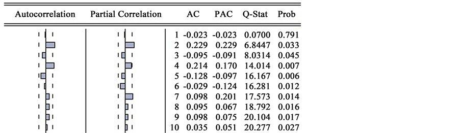
Figure 2. Self-correlation and partial self-correlation pictures of at most 10 orders in the steady sequence.
ups and downs is relatively accurate.
3.1.4. Contrastive Analysis
To inspect the superiority of the combined model, we also fit the price sequence respectively with ARIMA model and RBF neural network model. Relative errors of the predicting outcomes of the three models over the true values are in Figure 4. The relative error of ARIMA and RBF-ANN combined model indicated by full lines; relative error of ARIMA model indicated by dotted lines; relative error of RBF neural network model indicated by dots. Mean Absolute Percent Error (MAPE) of the predicted value of three models is indicated as Table 1 shows.
Clearly, the error fluctuation degree of ARIMA and RBF-ANN combined model proposed by this paper reaches the least and the prediction preciseness reaches the highest with the superiority.
Furthermore, the effects of further prediction on models are inspected. For the prediction of the data on the t-th day, the paper respectively uses the first t − 1, t − 2, t − 3 and t − 4 data as the training set for prediction. The obtained MAPE is shown as Table 2.

Figure 3. The true value curve, ARIMA model prediction curve and the combined model prediction curve.

Figure 4. The relative error picture of two single models and combined model.

Table 1. The respective MAPE values of two single models and combined model.
Table 2. Prediction preciseness of the combined model of different lag-phase training set that is used.
It can be seen that when the training set is lagged for above 2 phases, the forecast errors are obviously higher and the errors of the combined model are more than those of the ARIMA model. It fully verifies that the chaos characteristics of stock data increase dramatically as the forecast period goes up. The neural network model is more applicable to the capture of its short-term change rules. Therefore, it is right for the paper to choose to make short-term prediction on the future phase 1.
Furthermore, to inspect the effects of this paper to use multiple index combination input volumes such as the opening price, the highest and lowest price and transaction volume to enhance the prediction preciseness when constructing RBF neural network, the paper also carries out check experiments: only using the pure closing price sequence as the input volume to make combined model prediction under the same condition without considering other factors. Now, the predicted MAPE = 1.2624%, higher than the MAPE = 0.9071% predicted by the model in this paper. This means that the combination input added by this paper has effectively elevated the prediction accuracy and is totally necessary.
3.2. Prediction for Real Future
To make it meaningful, the paper also uses the combined model to predict the real future data, which is the closing price of November 2nd, 2015. The input data are the daily opening price, closing price, highest price, lowest price and transaction volume of 202 trading days from January 1st, 2015 to October 31st, 2015. The output price of the combined model is 3504.32. To apply this model for more future days, it has to take the dynamic prediction method illustrated in the part of model effectiveness test to predict future closing prices day by day.
4. Conclusion
Regarding the chaos and complexity of share price fluctuation, which possesses both linear and non-linear characteristics, it’s difficult to fit all the features of the information with single linear or non-linear prediction model. The paper proposes an ARIMA and RBF-ANN combined prediction model in which several prices and transaction volume indicators are chosen as combined input variables, hence endowing the model with high precision and good operability. An empirical study on short-term prediction on CSI 300 index is implemented to verify the superiority of the combined model over the other two, the precision of this combined model has obviously exceeded the single linear or non-linear model, as well as the prediction pattern with single closing price sequence as input variables. However the short-term prediction effects of the model are obviously better than long-term prediction effects, so relations between the share price and different factors, as well as the prediction on weekly and monthly data, have yet to be studied.
Cite this paper
LyuxunYang,XiCheng, (2015) Predictive Analytics on CSI 300 Index Based on ARIMA and RBF-ANN Combined Model. Journal of Mathematical Finance,05,393-400. doi: 10.4236/jmf.2015.54033
References
- 1. Bai, Y. (2009) Forecast and Analysis of Shanghai Stock Index Based upon ARIMA model. Science Technology and Engineering, 9, 4885-4888.
- 2. Ouyang, J. and Lu, L. (2011) Application of Integrative Improved BP Neural Network Algorithm in Stock Price Forecast. Computer and Digital Engineering, 39, 57-59.
- 3. Yang, X. (2014) Analysis on the Share Price Prediction Based on the Main Component and BP Neural Network. Statistics and Decision, 12, 42-43.
- 4. Hann, T.H. and Steurer, E. (1996) Much Ado about Nothing? Exchange Rates Forecasting: Neural Networks vs. Linear Models Using Monthly and Weekly Data. Neurocomputing, 10, 323-339.
http://dx.doi.org/10.1016/0925-2312(95)00137-9 - 5. Ediger, V., Akar, S. and Ugurlu, B. (2006) Forecasting Production of Fossil Fuel Sources in Turkey Using a Comparative Regression and ARIMA Model. Energy Policy, 18, 3836-3846.
http://dx.doi.org/10.1016/j.enpol.2005.08.023 - 6. Zhang, L., Cao, J. and Jiang, S. (2008) Practical Course of Neural Network. Beijing Mechanical Industry Press, Beijing.
- 7. Wei, M. and Yu, L. (2012) A RBF Neural Network with Optimum Learning Rates and its Application. Journal of Management Sciences in China, 15, 50-57.
- 8. Piggio, T. and Girosi, F. (1989) A Theory of Networks for Approximation and Learning. A.I. Memo No. 1140, Artificial Intelligence Laboratory, Massachusetts Institute of Technology, Cambridge.