Journal of Mathematical Finance
Vol.3 No.3A(2013), Article ID:38809,7 pages DOI:10.4236/jmf.2013.33A007
Cross-Market Valuation with Full Information on the Company’s Capital Structure
1Institute of Mathematics, University of Cologne, Cologne, Germany
2Institute of Finance, University of Ulm, Ulm, Germany
Email: pheider@math.uni-koeln.de, pposch@uni-bonn.de
Copyright © 2013 Pascal Heider, Peter N. Posch. This is an open access article distributed under the Creative Commons Attribution License, which permits unrestricted use, distribution, and reproduction in any medium, provided the original work is properly cited.
Received July 9, 2013; revised August 22, 2013; accepted September 7, 2013
Keywords: Credit Risk; Asset Pricing; CDS; Capital Structure; Equity Volatility
ABSTRACT
Most models for forecasting a company’s value either use only information from single markets or compress information from other markets. We propose a model using a company’s full capital structure including the term structure and type of outstanding debt to assess its future value. We discuss the numerical properties of our model and demonstrate its usefulness when estimating the probability of default as a valuation example.
1. Introduction
There is a variety of theoretical and empirical work using market data to price the equity or the credit side of a company. However, there are few attempts to use all available information of a company’s capital structure. Broadly speaking, a firm’s financial resources are divided into equity and debt, where the former is traded through the stock of the company and the latter is available to debt holders through loans, bonds or structured debt vehicles, e.g. asset backed securities. With the evolution of the credit default swap market, there has been a third information source, solely used by professional traders and thus considered very efficient in pricing a company’s default risk.
Including more market information increases the precision of any estimate as even when we assume a market to be strongly efficient and the observed market price reflects all available information, it is not wise to neglect additional prices from other markets. For example, considering a senior bond investor, the price of her position in an efficient market reacts to a deterioration of the company’s creditworthiness only up to the level of the expected recovery of the bond. The equity piece, in contrast, is fully exposed to a credit event leading to more pronounced reactions in the company’s stock price. Combining the information from both markets, the bond and the stock price dynamics, increases the validity of any valuation.
The empirical literature related to our approach discusses interactions between two markets. [1] shows credit markets to lead bond markets and both lead rating information in default prediction. [2] establishes the link between equity volatility and credit default swaps, [3] relates the former market to bond yields and [4] looks into the determinants of credit spreads. Furthermore, there is a variety of very detailed and insightful work on single markets and their different aspects. On the theoretical literature brand, we employ the structural model class proposed by [5] and its more operational version by [6] and use straightforward method to extract default probabilities from bond prices, e.g. [7-9].
The combination of these models allows us to use all available information on the company’s financial situation such as balance sheet information, stock price dynamics, debt structure, debt maturity, term structure and market prices of default risk. It is crucial to note that assessing a company’s default risk is only one of the applications of our model. It can also be used as a pricing tool for any of the three markets, as a company valuation approach or to spot differences in the market’s valuation in a capital structure arbitrage setting.
In the next section, we will introduce our model. The implementation and results of the model are then subjected to the third section, while the last part concludes.
2. Model
Fundamental to our model is the filtered probability space  under the martingale measure
 . The filtration
  is assumed to satisfy the usual conditions. We focus on the equity, bond and default risk dynamics of a company.
Let  be a time horizon and we denote by time
  today. We assume that the capital structure of the company is changed at known, discrete times
which are for example bond redemption dates, coupon dates, future bond emissions or changes in the loan structure of the company. At these days we allow for changes in the debt structure of the company. In our implementation these dates will be derived from the bond and loan structure of the company. For example IBM currently has 24 bonds outstanding resulting in an average time between bond events of nine days. We assume that the debt is constant in between two  and
and  and denote the outstanding debt on a per share basis by
 .
.
One particular important application of a company’s valuation is the assessment of its likelihood to fail on fulfilling its financial obligations. While there are several ways to model the default probability  of a default of the company between t and a later time
  we propose a combination of common approaches of default risk modelling to obtain model of equity dynamics.
We use an intensity based default model and a [5] type default model to obtain equity volatilities. The tenor structure  of capital structure dates together with the prevailing debt-per-share ratios
  at dates
  will induce a term structure of equity volatilities
  and consequently a term structure of implied stock volatilities
 . Based on this set of volatilities we model the equity price process.
In our structural model we use standard assumptions to derive the survival probability  for a company. With this measure at hand we can both assess the riskiness of the company as well as induce its market prices. The latter is found by the fundamental link between the riskiness of the company and the compensation demanded by both equity and bond holder to hold the company’s assets. We will illustrate this link in the empirical section of this paper, now for the theory we model the company’s asset value V under the measure Q as a geometric Brownian motion
where the asset volatility  is unknown. There is an extensive literature extending this type of models with more stochastic, however the trade-off between a theoretically more appealing and a traceable model is large. We use a model variant proposed by [6] with some of the extensions applied, especially the implementation of implied volatility and implied leverage based on [10,11].
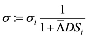
The recovery rate  and its volatility
  can be based on recovery statistics published by rating agencies. Alternatively, option implied volatilities can be used, we will demonstrate the latter in the empirical section. The unobservable asset volatility
  is related to the observable equity volatility
  by
by
 (2.1)
(2.1)
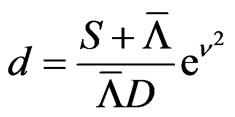
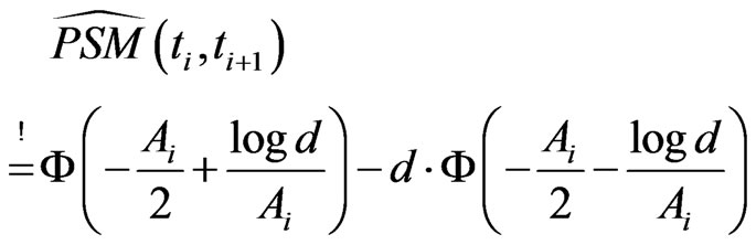
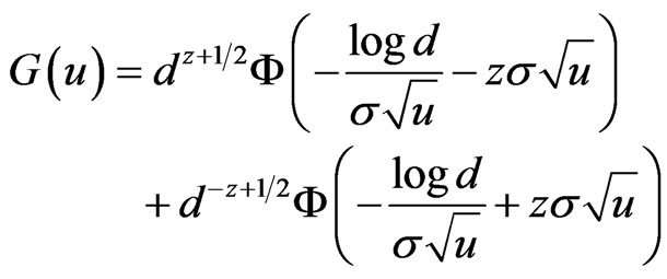
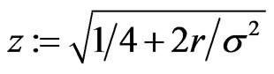
The approximate survival probability  depends on
 ,
,  ,
,  ,
,  ,
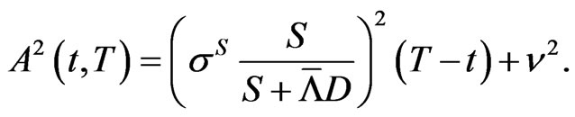
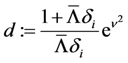
,  and is given as
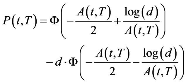 (2.2)
(2.2)
with
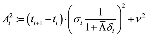
Our first goal is to obtain an implied equity volatility term structure together with a term structure for the debt per share ratio. These volatilities mimic the company’s riskiness using full market information.
For the tenor structure 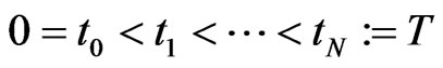 and each time interval
  we estimate the stock volatility
in that time interval and the debt per share ratio
The resulting term structure  and
and  will be denote by bold letters in the following and generally, we will denote any term structure by bold letters in the following.
For example, it makes sense for an investor to monitor the future development of a company (in terms of volatility and debt per share ratio) quarter-annually over the investment horizon .
.
We combine information from several observable markets, the bond market, CDS market and stock option market. Each market contains information and market expectations for the future, which are the implied hazard rates from the bond market, the default expectations from the CDS market and the implied volatilities from the option market each seen from today . In detail, we collect 1) for
  the cumulative default probability
  between 0 and
 2) for
  the cumulative survival probability
  between 0 and
 3) for
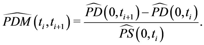
  the marginal default probability
  between
  and
and  conditional on no default till
 . It is,
Further, this gives 4) for  the marginal survival probability
  between
  and
and  conditional on no default till
 5) for
  the CDS-spread
  with maturity
 6) for
  the marginal CDS-spread
  between
  and
and 7) for
  implied volatilities
  of observable ATM options with maturities
 .
.
Remark: Because the bond-tenor structure  and CDS-tenor structure
  does not match neccessarily the tenor
  we use appropriate interpolation methods to strip all necessary data from observable bond and CDS data.
The backbone of the model is the linkage of all these markets by the structural model discussed above. We proceed recursively and determine the unknown values  and
and  step by step. We start with
  and proceed with the following computational step successively:
step: :
:
Goal: Find  and
and .
.
Solve system for the unknown ,
, :
:
 (2.3)
(2.3)
with
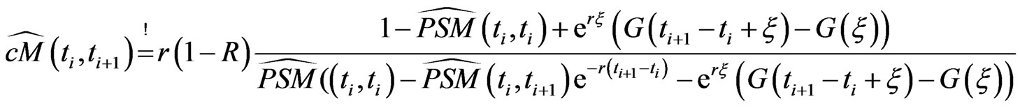
and Equation (2.4)
with
for unknown  and
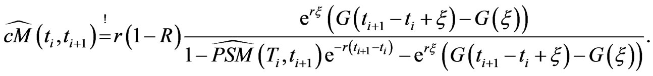
and , cf. [6]. Assuming
  , this simplifies to Equation (2.5).
The right hand side of this system stems from Equation (2.2) adapted to a time period . Hence, we equal the model implied marginal CDS spread and the observed marginal CDS spread and also the marginal survival probabilities. To stabilize the numerical process we use the observed marginal probability in the right hand side of Equation (2.4). Moreover, instead of a root finding algorithm to solve the system we use a minimization to find
  and
and  in each step which increases the numerical robustness of the iteration step.
At this stage of the procedure only CDS data and bond data are involved in the determination of the term structures  and
and . Denote by
 and
and
 the observed marginal survival probabilities and CDS-spreads. We can interpret the above recursive computation as a mapping from the space of observables
  to the space of term structures
 ,
,
However,  and
and  are not observable in the real world, so that the model cannot be calibrated in its current form and we need a further mapping to observable market data.
With given volatility term structure  we can compute by Black-Scholes formula option prices and obtain implied volatilities for all traded options. Since our volatility term structure is deterministic in the strike direction
 (2.4)
(2.4)
 (2.5)
(2.5)
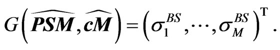
we will not observe a volatility smile, yet curvature in the maturity direction can be modelled. Therefore, we fix a level of moneyness and stick with at-the-money (ATM) options. Hence, we can project the unobservable  onto observable Black-Scholes ATM-implied volatilities
  for observable options with maturities
 . In this way we managed to define a mapping
  from the space of observables
  to the space of observable ATMimplied volatilities,
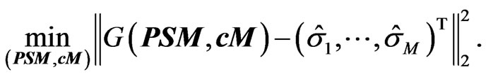
Assuming only mispricing in the CDS and bond market, i.e. no mispricing in option market, we can identify mispricing by the least-squares approach
More realistic is to assume also mispricing on the option market. Hence, we have to include the ATM-implied volatilities in the minimization process. Therefore, we suggest to minimize the following functional
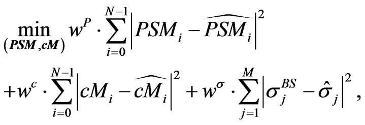 (2.6)
(2.6)
where  are weights and scales to reflect our assumptions on the quality of the observed market prices.
3. Numerical Study
Before we test our setup on real world data we perform a couple of test cases. We assume for all cases a constant risk-free rate , no dividend,
  ,
,  and bond/CDS recovery rate
 . We will monitor quarter annually and assume a stepwise hazard rate
  for the the interval
 . From hazard rates we get by the credit triangle,
and
with .
.
Assume that we have stripped from the bond market the hazard rates  and from the CDS market the rates
 .
.
Case 1: In our first test scenario we assume that bond and CDS market imply the same hazard rates, hence . Further, we assume that the rates are flat for each year with jumps at the end of each year. In particular, consider
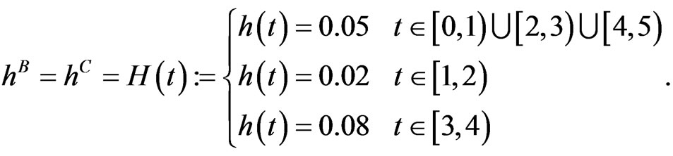
From  we get
  and
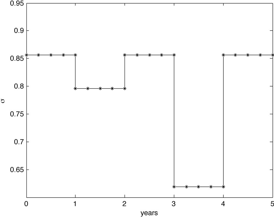
and  and compute the volatility and debt per share term structure, see Figure 1. Seen from
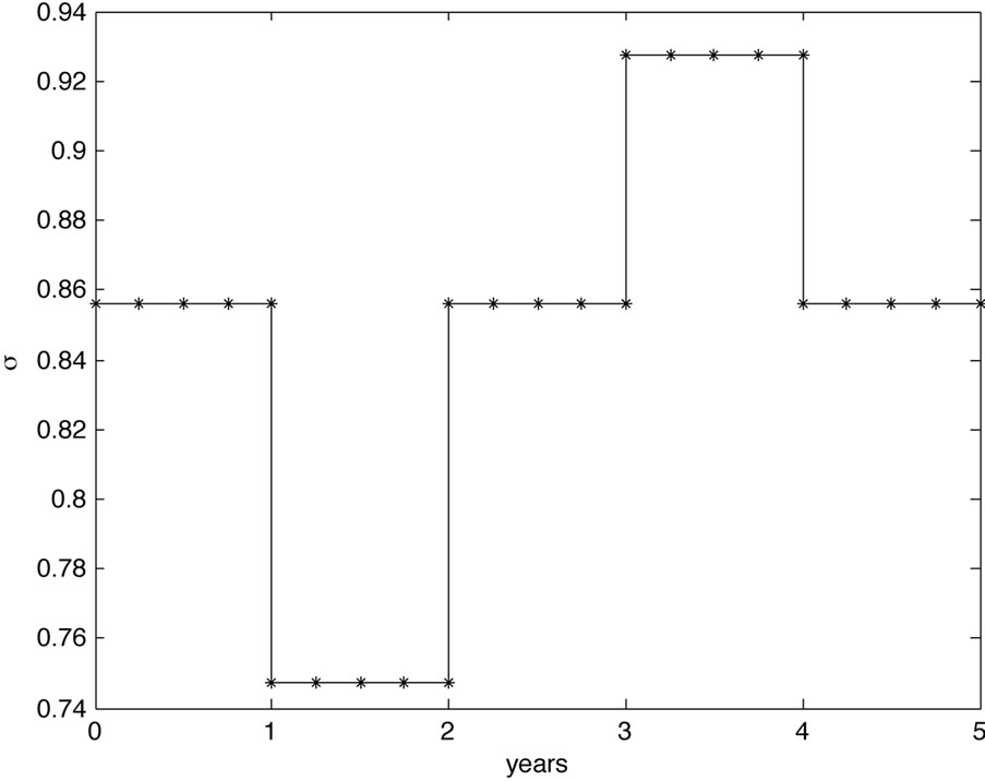
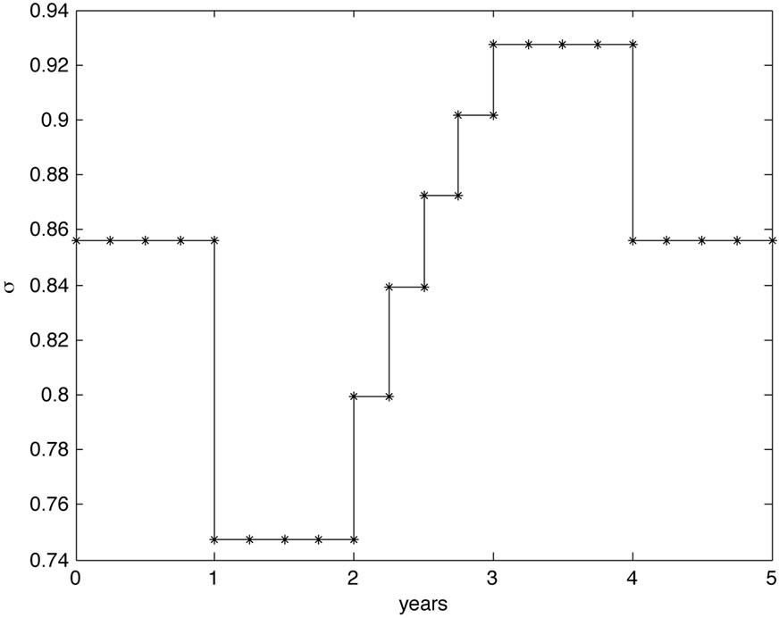
 , the term structures suggest a drop in volatility in the second year and a rise in volatility for the fourth year, seen from the level of the first year. This corresponds to the lower resp. higher level of hazard rates during these time periods. Further, if we assume a constant level of equity then the debt per share ratio suggests lower debt in the second year and increasing debt in the fourth year with respect to the debt level at the beginning in accordance to the lower resp. higher hazard rates. For example, the decrease in debt in the second year results in a shortage of outstanding bonds, that is rising bond prices which is reflected in lower hazard rates.
 (a) Volatility term structure
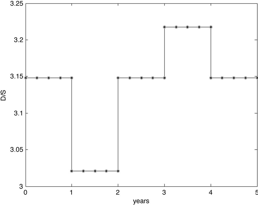 (b) Debt per share term structure
Figure 1. Volatility and debt per share term structure for study Case 1.
Case 2: For the second scenario we assumed a flat hazard rate  from the CDS market throughout the 5 years, and
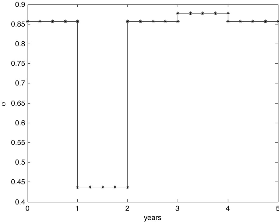
  for the rates from the bond market. Hence, the market implies a constant default risk for the company for the next 5 years. For the second year we assumed an increase in bond prices that is a drop in the risk premium for the company implied from debt and we expect a drop in volatility due to a less risky company and a drop in debt per share ration as less debt is outstanding on the market. In the fourth year we assumed more risk stemming from the bond market. Yet, the default risk is untouched showing a strong market belief in this company resulting in a drop of volatility. On the other hand rising risk premiums from the bond market signal more debt and we expect a rising debt per share ratio. The model results are shown in Figure 2.
Case 3: For the third scenario we assumed a flat hazard rate  from the bond market throughout the 5 years, and
  for the rates from the CDS mar-
 (a) Volatility term structure
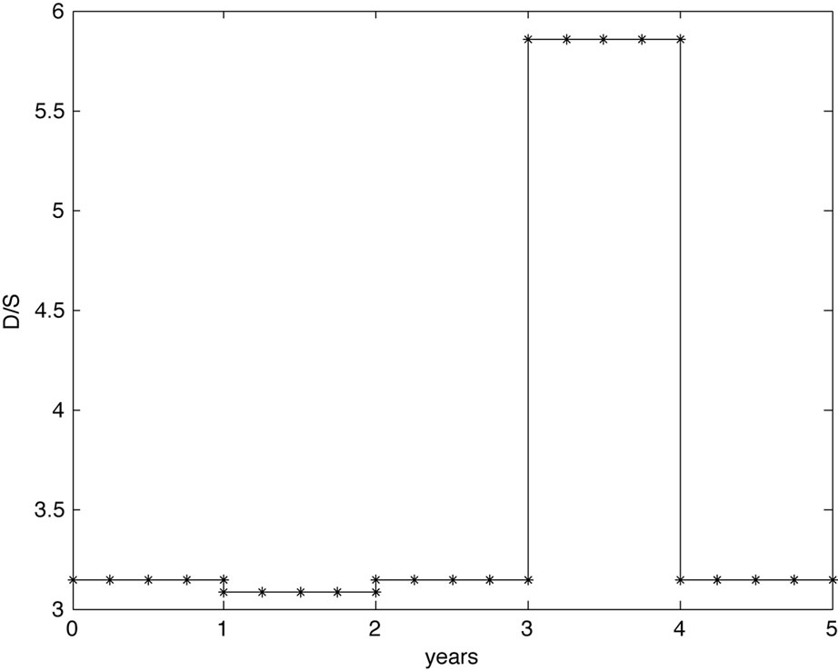 (b) Debt per share term structure
Figure 2. Volatility and debt per share term structure for study Case 2.
ket. Quantitatively, if default risk drops and bond risk stays untouched, one expects the volatility to drop as well as there is less risk in the underlying. Because there is a mismatch between the CDS implied default risk of the company, which is low for the second year, and a higher level of risk premium from the bond market, there is a strong market belief in the company and a rise in the debt per share ratio. On the other hand, rising default risk in the fourth year implies a higher volatility. The cause of the higher default risk is explained by a higher degree of debt. The model results are shown in Figure 3.
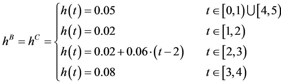
Case 4: For the last example we extend our previous hazard rate by a linear increase in the third year,
 (a) Volatility term structure
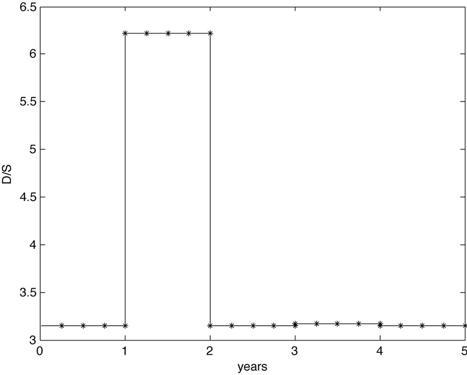 (b) Debt per share term structure
Figure 3. Volatility and debt per share term structure for study Case 3.
and assume that bond and CDS market follow this hazard rate. Hence, the risk is determined by the hazard rate which is reflected in the volatility mimicking the behavior of the hazard rate, see Figure 4. Moreover, we would also expect that the debt per share ratio mimics the hazard rate as the debt level is determined by the bond prices.
We finish this section with a real-world example. For our study we took the  as observation day and chose IBM company as underlying because options on IBM and CDS quotes are liquidly traded and IBM offers a rich structure of issued bonds with different maturities. We assume a constant risk free interest rate of 1.5% to simplify discounting, a mean standard deviation of the global recovery
  and a percentage standard deviation of the global recovery
  in the CreditGrades model. From bond market we picked three bonds
 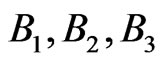 with maturities
  and CDS quotes with maturities 6 m, 1 y, 2 y which are tabulated in Table 1.
 (a) Volatility term structure
 (b) Debt per share term structure
Figure 4. Volatility and debt per share term structure for study Case 4.
From the bond data we stripped observed marginal survival and default probabilities between the given time points and obtained marginal CDS quotes by assuming a flat hazard rate between two successive time points from the observed CDS quotes. The results are summarized in Table 2.
From option quotes we collected data for ATM options with maturities 30 d, 3 m, 6 m, 12 m, 18 m, see Table 3. We assume that all input data might be inflicted by mis-pricing so that we choose Equation (2.6) for the calibration with weights . The optimization was done by Nelder-Mead algorithms which avoids the computation of derivatives and works very robustly even in higher dimensions [12].
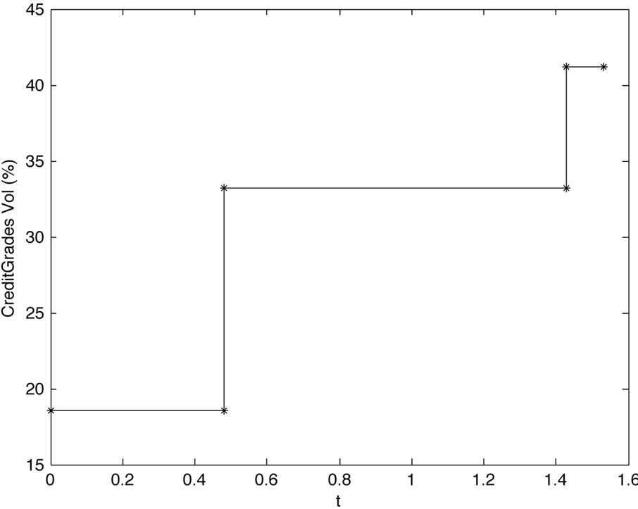
The results of the calibration is summarized in Figure 5 which shows the model implied volatility and debt per share term structure. Hence, the model implies rising riskiness of IBM over the next one and a half year, and a drop of the debt per share ratio beginning in 6 month and lasting for about one year. From the volatility term structure in Figure 5 we get Black-Scholes implied ATM volatilities for options with different maturities. We compare the model implied ATM volatilities to the market observed data in Table 3. We observe that the short term options (i.e. maturity till 6 month) are matched well by the model whereas the model suggest higher implied volatilities for the long term options (12 months and 18 months) in accordance to the volatility term structure in Figure 5.
Moreover, we get marginal credit default swaps and default probabilities by the calibration. For a comparison we calculated from the computed marginal spreads the model implied CDS quotes for 6 m, 1 year and 2 years, see Table 1. In good accordance to the above results the
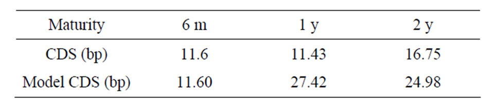
Table 1. Observed CDS and model implied CDS quotes.
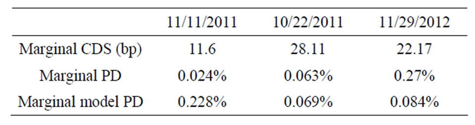
Table 2. Marginal CDS quotes, survival and default probabilities and model implied marginal probabilities.
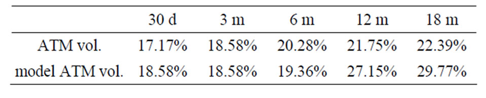
Table 3. Observed ATM implied volatilities and model implied volatilities.
 (a) Volatility term structure
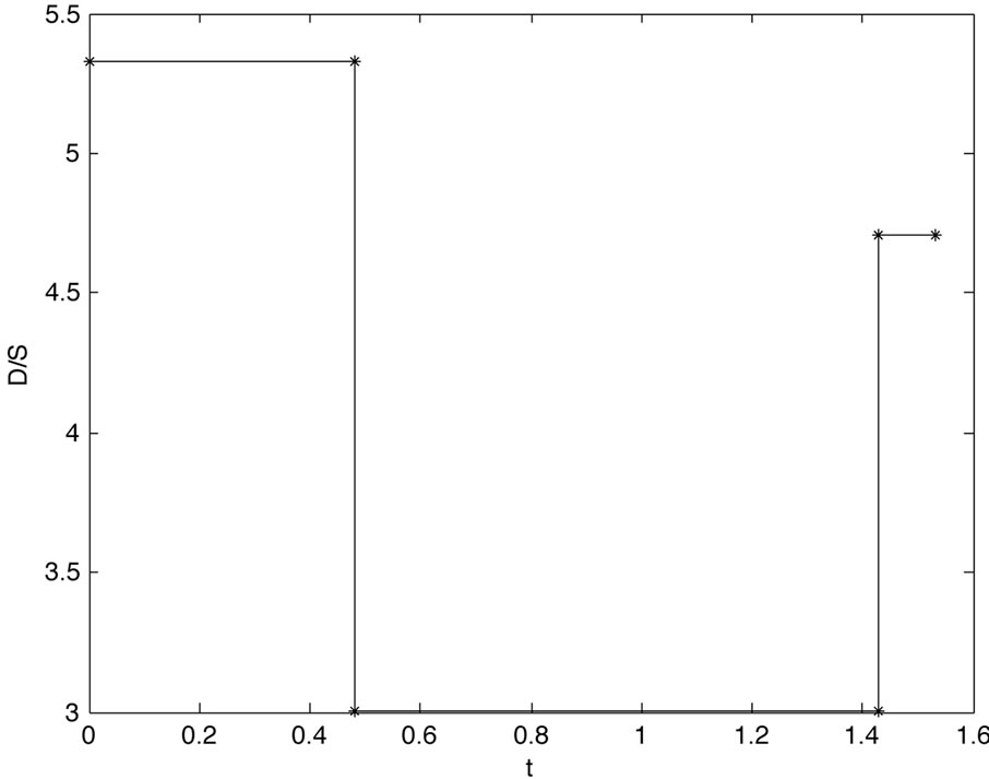 (b) Debt per share term structure
Figure 5. Volatility and debt per share term structure for IBM with observation day T0 = 5 = 18 = 2011.
model implies higher risk levels of IBM starting in 6 months. The calibrated marginal default probabilities are shown in Table 2. They are matching the observed data well.
4. Conclusion
Precise estimation of market parameters is crucial for a variety of applications. Regulatory bodies, for example, rely on default estimates from rating agencies or implied measures from single markets. Combining all available information within one structural approach enables market participants to benefit from the full information set. In the example of default estimates, the outcome is more precise and stable over time compared with a single market’s outcome. We use widely-accepted models for the equity and credit side of a company and combine them into a single model. We demonstrate the numerical properties of our model and estimate an example. Future research should focus on a broad market study and a full benchmark against more simple models.
REFERENCES
- J. Hull, A. White and M. Predescu, “The Relationship between Credit Default Swap Spreads, Bond Yields, and Credit Rating Announcements,” Journal of Banking & Finance, Vol. 28, No. 11, 2004, pp. 2789-2811. http://dx.doi.org/10.1016/j.jbankfin.2004.06.010
- B. Y. Zhang, H. Zhou and H. Zhu, “Explaining Credit Default Swap Spreads with the Equity Volatility and Jump Risks of Individual Firms,” Review of Financial Studies, Vol. 22, No. 12, 2009, pp. 5099-5131. http://dx.doi.org/10.1093/rfs/hhp004
- J. Y. Campbell and G. B. Taskler, “Equity Volatility and Corporate Bond Yields,” The Journal of Finance, Vol. 58, No. 6, 2003, pp. 2321-2350. http://dx.doi.org/10.1046/j.1540-6261.2003.00607.x
- P. Collin-Dufresne, R. S. Goldstein and J. S. Martin, “The Determinant of Credit Spread Changes,” The Journal of Finance, Vol. 56, No. 6, 2001, pp. 2177-2207. http://dx.doi.org/10.1111/0022-1082.00402
- R. C. Merton, “On the Pricing of Corporate Debt: The Risk Structure of Interest Rates,” Journal of Finance, Vol. 29, 1974, pp. 449-470.
- C. C. Finger, V. Finkelstein, G. Pan, T. Ta, J.-P. Lardy and J. Tierney, “Creditgrades,” Technical Report, RiskMetrics Group, Inc., 2002.
- J. Hull, “Options, Futures, and Other Derivatives,” Prentice Hall, Upper Saddle River, 2008.
- D. Xu and F. Nencioni, “Introducing the jp Morgan Implied Default Probability Model: A Powerful Tool for Bond Valuation,” JP Morgan Research, 2000.
- J. Hull, M. Predescu and A. White, “Bond Prices, Default Probabilities and Risk Premiums,” Journal of Credit Risk, Vol. 1, 2005, pp. 53-60.
- J. Hull, A. White and I. Nelken, “Merton’s Model, Credit Risk and Volatility Skews,” Journal of Credit Risk, Vol. 1, 2005, pp. 1-27.
- R. Stamicar and Ch. C. Finger, “Incorporating Equity Derivatives into the Creditgrades Model,” Riskmetrics.com, 2005.
- J. A. Nelder and R. Mead, “A Simplex Method for Function Minimization,” Computer Journal, Vol. 7, No. 4, 1965, pp. 308-313. http://dx.doi.org/10.1093/comjnl/7.4.308