Journal of Mathematical Finance
Vol.3 No.2(2013), Article ID:31827,16 pages DOI:10.4236/jmf.2013.32029
A Liability Tracking Approach to Long Term Management of Pension Funds
1Graduate School of Innovation Management, Tokyo Institute of Technology, Tokyo, Japan
2The Government Pension Investment Fund, Tokyo, Japan
Email: ieda@craft.titech.ac.jp
Copyright © 2013 Masashi Ieda et al. This is an open access article distributed under the Creative Commons Attribution License, which permits unrestricted use, distribution, and reproduction in any medium, provided the original work is properly cited.
Received May 28, 2013; revised July 2, 2013; accepted July 11, 2013
Keywords: Pension Fund Management; Long Term Portfolio Optimization; Quadratic Hedging; Stochastic Optimal Control; Hamilton-Jacobi-Bellman Equations; LQG Control
ABSTRACT
We propose a long term portfolio management method which takes into account a liability. Our approach is based on the LQG (Linear, Quadratic cost, Gaussian) control problem framework and then the optimal portfolio strategy hedges the liability by directly tracking a benchmark process which represents the liability. Two numerical results using empirical data published by Japanese organizations are served: simulations tracking an artificial liability and an estimated liability of Japanese organization. The latter one demonstrates that our optimal portfolio strategy can hedge his or her liability.
1. Introduction
In the management of pension funds, a long term portfolio strategy taking into account a liability is one of the most significant issues. The main reason is the demographic changes in the developed countries: if the working-age population is enough to provide for old age, the liability is a minor issue in the portfolio management of pension funds. Since the life expectancy have increased in recent decades, it becomes insufficient to provide for old age. Furthermore the low birth rate continues and drives up this problem for decades. Thus pension funds face a challenging phase to construct long term portfolio strategies which hedge their liabilities.
A lot of pension funds except a few ones [1] determine their portfolio strategies by the traditional single time period mean variance approach which excludes an evaluation of a liability. Its intuitive criterion attracts managers of pension funds. However the single time period approach is unsuitable for a long term portfolio management in the sense that it is unable to change the strategy excepting the initial time. The multi time period approach which arrows the change of the strategy has a problem that the computational complexity grows exponentially. Hence if we employ this approach, we are usually unable to obtain the optimal portfolio strategy in realistic time.
Therefore the aim of this paper is to propose a long term portfolio strategy which 1) involves an evaluation of a liability, 2) admits changes of the strategy at any time, and 3) is obtained in realistic time. To tackle this problem, we employ the LQG (Linear, Quadratic cost, Gaussian) control problem (see, e.g., Fleming and Rishel [2]). The LQG control problem is a class of stochastic control problem and is able to provide the control minimizing the mean square error of a benchmark process and a controlled process. Roughly speaking our tactic is that we compute the optimal portfolio strategy with the benchmark process which represents the liability. Then we can track the liability by using our optimal portfolio strategy. Although it is difficult to obtain the solution of stochastic control problem in general, the LQG control problem has the analytical solution which assures that we are able to obtain the solution in realistic time and thus it meets our purpose.
A continuous time stochastic control approach is one of the most popular method to obtain the suitable long term portfolio strategy. The literature about this approach is quite rich. The papers treating the management of pension funds are, for instance, as follows: Deelstra et al. [3] and Giacinto et al. [4] discuss the portfolio management for pension funds with a minimum guarantee; Menoncin and Scaillet [5] and Gerrard et al. [6] deal with the pension scheme including the de-cumulation phase. Our study is on the cutting edge in the sense that deal with tracking liabilities directly and constructing a suitable long term portfolio at the same time.
The organization of the present paper is as follows. We introduce continuous time models of assets and a benchmark in Section 2. To fit in the LQG control problem, they are defined by the linear stochastic differential equations (SDEs). We mention that our portfolio strategy is represented by the amounts of assets. In Section 3, we define a criterion of the investment performance and provide the optimal portfolio strategy explicitly. Several numerical results are served in Section 4 Throughout the section the parameters related to the assets are determined by an empirical data provided by the Government Pension Investment Fund in Japan. The simulation using an artificial data are discussed in Section 4.1 and this result gives conditions that our optimal portfolio strategy works well. Section 4.2 provides a case study using an empirical estimations published by the Japanese Ministry of Health, Labour and Welfare. It demonstrates that our strategy is able to hedge the liability well.
2. Continuous Time Models of Assets and a Benchmark
In this section, we present mathematical models of assets and a benchmark. The market which we are considering consists of only one risk-free asset and  -risky assets and we have
  -benchmark component processes.
Let  be a filtered probability space
  be a
be a  -dimensional Brownian motion where
  and
and  be a space of stochastic processes
  which satisfy
We denote price process of the risk-free asset, those of the risky assets and the benchmark component processes by ,
, and
and  respectively, where the asterisk means transposition. To fit in the LQG control problem, we assume that
 ,
, and
and  are governed by the following SDEs:
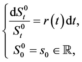 (1)
(1)
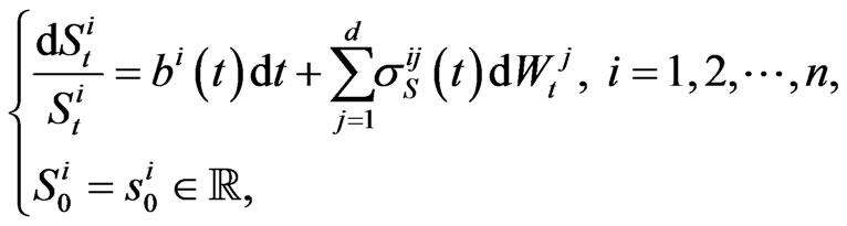 (2)
(2)
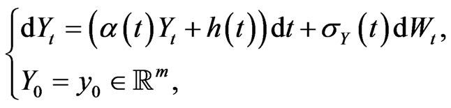 (3)
(3)
where ,
,  ,
,  ,
,
 ,
,  and
and
 are deterministic continuous functions and
  represents the maturity. Coefficients
 ,
,  and
and  stand for the risk-free rate and the expected return rate of the
  -th asset and the volatility.
Let a class of portfolio strategy  be the collection of
  -valued
  -adapted process
  which satisfies
 be the amount of the risky asset held by an investor at time
 , and
, and  be the value of our portfolio at time
 . Then the amount of the risk-free asset held by the investor is represented by
 . Hence,
  is governed by
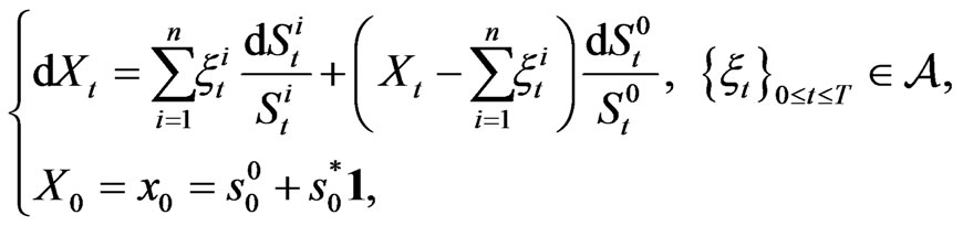 (4)
(4)
where . To emphasize the initial wealth and the control variable, we may write
 .
.
The solution  of the SDE (4) is given as follow:
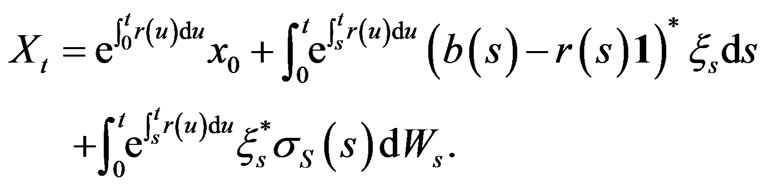
Moreover since ,
,  , and
, and  are continuous functions on
  and
and ,
,  is in
is in :
:
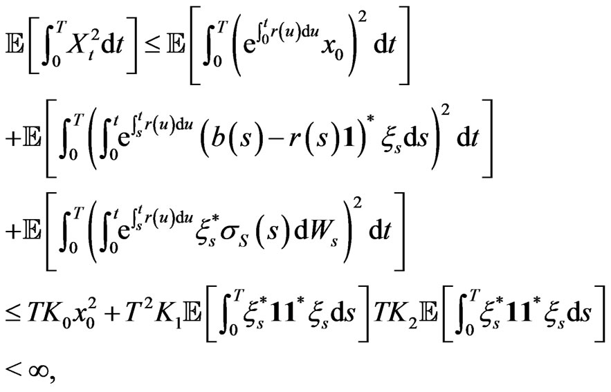
where ,
,  and
and  are constants.
3. Optimal Investment Strategy
We define the criterion of investment performance  by
by
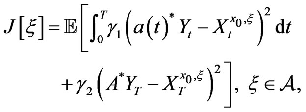 (5)
(5)
where  and
and  are constants,
  is a constant vector, and
  is a deterministic continuous function. Hence our investment problem is to find the control
  s.t.
s.t. ,
, . Since the performance criterion is represented by quadratic functions, our investment problem becomes the LQG control problem. We determine
 ,
,  and the parameters of
  to be able to regard
  and
and  as a liability.
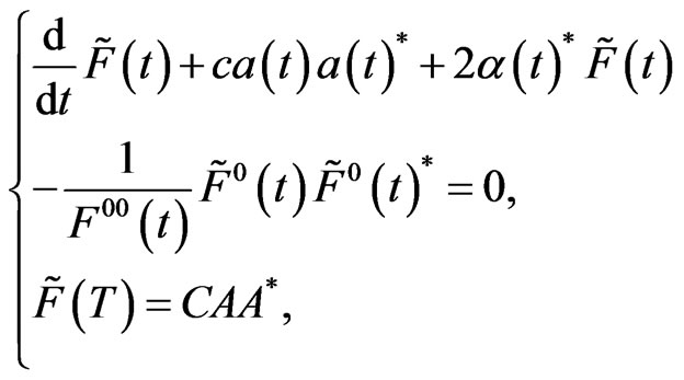
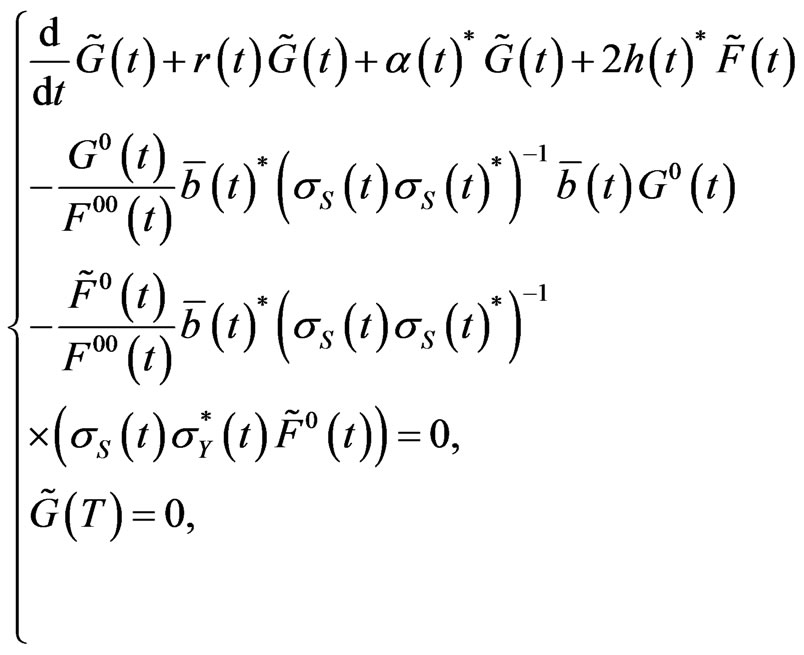
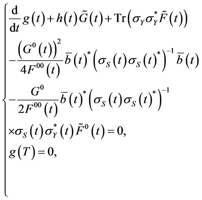
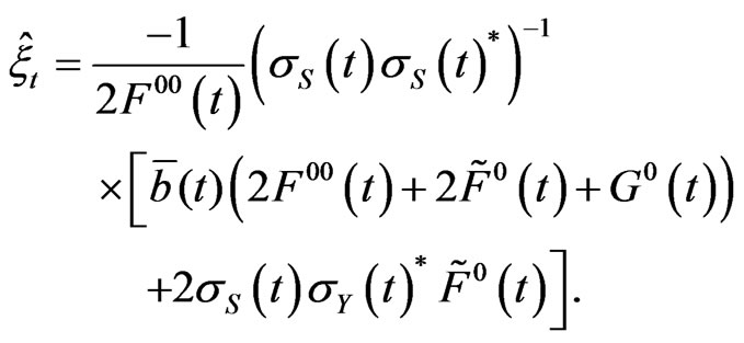
The optimal portfolio strategy is represented in the following form:
Theorem 1 We define the portfolio strategy  as follows:
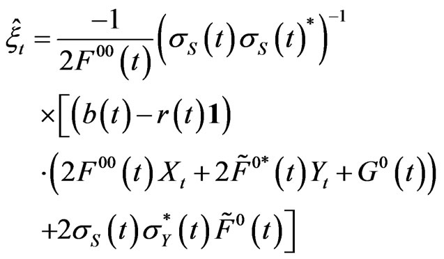 (6)
(6)
where  and
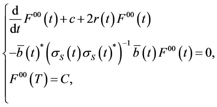
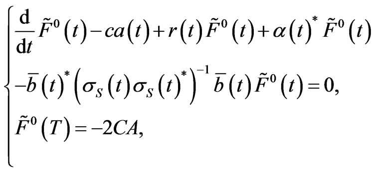
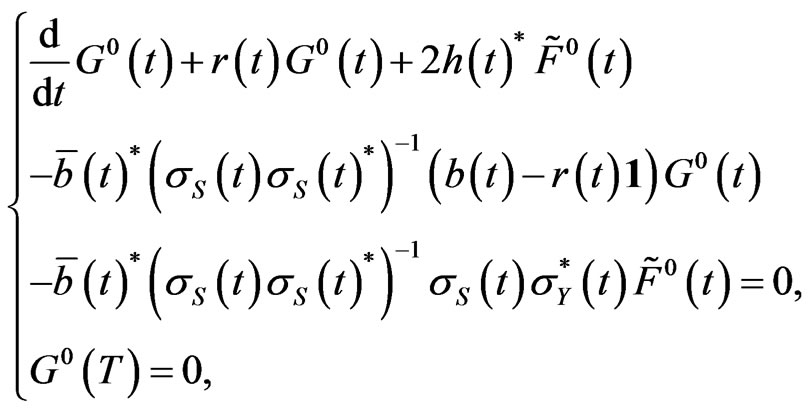
and  are solutions of following ordinary differential equations (ODEs):
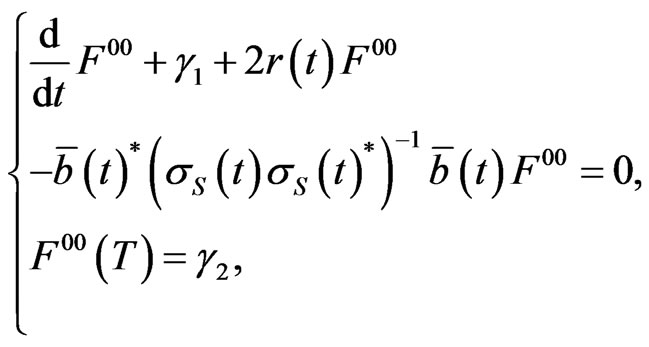 (7)
(7)
 (8)
(8)
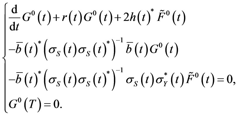 (9)
(9)
Here we have written .
.
Then  satisfies
  and
and ,
, .
.
The proof of Theorem 1 is given in the appendix.
We note that  has feedback terms of
  and
and . This implies that our optimal strategy has delays to catch up the the benchmark process
 . Hence the preferable situation applying our strategy is the case that
  does not fluctuate violently.
4. Numerical Results
We apply our method to an empirical data provided by the Japanese organizations. This section is divided to two subsections according to the type of liabilities: an artificial liability and the liability constructed by the estimations published by the Ministry of Health, Labour and Welfare of Japan. The former one suggests the situation that our optimal strategy works well and the latter one demonstrates that our portfolio strategy is able to hedge the liability.
Before we move on the each subsection, we determine the common parameters in following subsections. The first task is to determine the parameters relating to the benchmark component processes. They consist of the income of a pension fund  and his or her expense
  and thus
  and
and . We set the parameters constructing the benchmark process as follows:
Hence, the benchmark process is  which represents a shortfall of the income and then we regard this shortfall as the liability. To discuss the performance of the strategy, we introduce a hedging error function of the
  -th sample path
  and its average
  as follows:
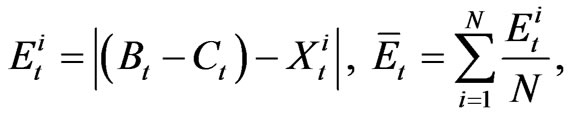
where  is the
  -th sample path of
  and
and  is the number of the sample paths. We set
  except as otherwise noted.
The next task is to determine the risk-free rate and the expected return rates and volatilities of risky assets. We invest the following four assets: indices of the domestic bond, the domestic stock, the foreign bond and the foreign stock; we number them sequentially. According to the estimations of return rate and volatilities by the Government Pension Investment Fund in Japan [7], we construct  and
and  as follows:
 ,
,  ,
,  and
and ;
;
 (10)
(10)
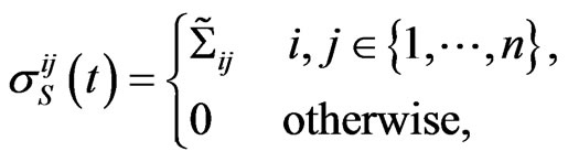
where  the Cholesky decomposition of
 , a variance-covariance matrix of the assets:
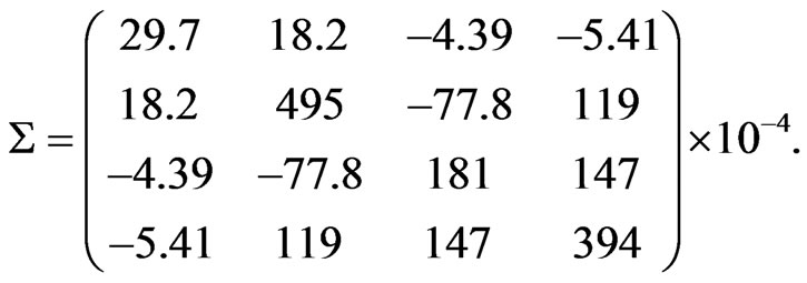
We choose a money market account as the risk-free asset and we set .
.
4.1. Simulation with an Artificial Liability
In this subsection, we consider the following an artificial deterministic liability model:
 (11)
(11)
 (12)
(12)
i.e., we set  and
and . We assume that our wealth coincides with the benchmark at the initial time:
 . We construct the optimal portfolio strategy over three decades, i.e.,
 . Then we determine the functions
 ,
,  and
and  by solving the ODEs (7)-(9) numerically. and simulate
  paths of
  on
on  according to Equations (1)-(3) using a standard Euler-Maruyama scheme with time-step
 . Figure 1 describes an investment result of a sample path. The black and red lines in Figure 1 represent
  and
and  respectively.
The most significant issue it indicates is that the performance of the strategy is quite poor near the maturity. Figure 2 describing  implies that this poor performance does not depend on the sample path. Figure 3 suggests a key factor of this phenomenon: values of functions
 ,
,  and
and  change drastically between
  and
and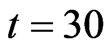 ; this time period coincides with the term the hedging error becomes large rapidly. Figure 3 also implies that the existence of the stationary solutions of the ODEs (7)-(9). As described in Figure 2, the strategy relatively works well on the time period when the functions
 ,
,  and
and  reach the stationary state. Hence the strategy will be improved by using the stationary solutions of the ODEs (7)-(9) on entire region.
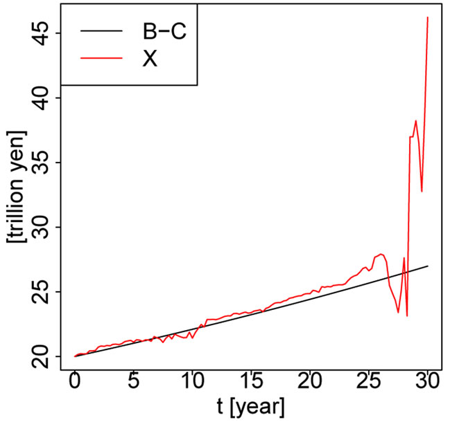
Figure 1. A sample path of  and
and . The black and red lines represent
  and
and  respectively.
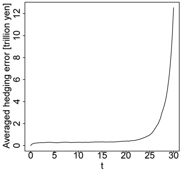
Figure 2. Averaged hedging error .
.
Figure 3. The time evolution of ,
,  and
and . The black, red, green and blue lines represent
 ,
,  ,
, and
and  respectively.
To obtain the stationary solutions of the ODEs (7)-(9), we replace  to a value large enough. We denote it by
  and set
 . Figure 4 shows values of
 ,
,  and
and  obtained by solving the ODEs (7)-(9) with parameter
 . We can find that the functions
 ,
,  and
and  take the stationary solutions on
 .
.
Results of simulations using the improved strategy are described as follows.
Figures 5 and 6 indicate that the performance near the maturity is improved and it does not depend on the sample paths. This result leads us to the conclusion that we should construct the strategy with the stationary solutions of the functions ,
,  and
and  if they exists.
At the end of this subsection, we mention about our portfolio composition. Figure 7 displays the asset allocation on the sample path described in Figure 5. The money market account, the domestic bond and the foreign stock indicated by light blue, black and blue lines respectively dominate our portfolio. The optimal strategy is that we keep the most part of the wealth as the money market account and compensate for the increment of the benchmark by the investment for the domestic bond, low risk and low return asset, and the foreign stock, high risk
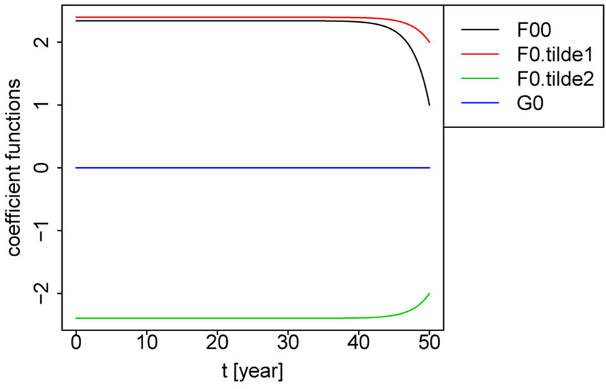
Figure 4. The time evolution of ,
,  and
and  (improved case). The black, red, green and blue lines represent
 ,
,  ,
, and
and  respectively.
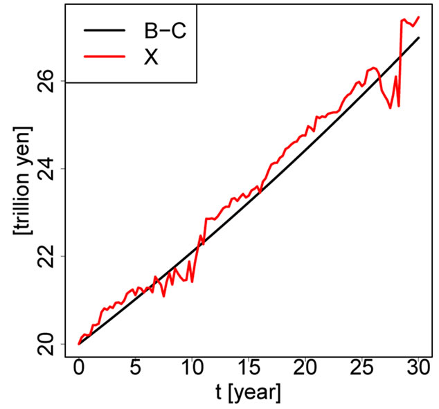
Figure 5. A sample path of  and
and  (improved version). The black and red lines represent
  and
and  respectively.
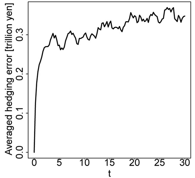
Figure 6. Averaged hedging error  (improved version).
and high return asset. If  is deficient in
 , the strategy increases the proportion of the domestic bond and the foreign stock.
4.2. Simulation with an Empirical Liability
According to the Japanese actuarial valuation published in 2009 [8], the estimated income and expense of the welfare pension are showed in the Figure 8.
We regard these estimations as  and
and  and simulate the three decades investments using our optimal strategy from 2040 when the shortfall of the pension fund starts to expand drastically. The following reasons support that this situation is a valid case study: 1) a phase expanding
 , the shortfall of the pension fund, is the most typical one expressing the demographic changes; 2) the behaviour of
  in this term meets the condition to apply our optimal strategy:
  is increasing in the entire region. Throughout this subsection we set the start point as the year 2040, i.e.,
  and
and  represent the year 2040 and the year 2055 respectively.
To construct the optimal strategy, we first calibrate ,
,  and
and  to fit the estimations. Setting
  and
and  as a numerical differentiation of the estimations is a simple method to accomplish the purpose. Since we are discussing the three decades portfolio, we determine
 . As suggested in Section
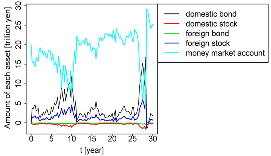
Figure 7. An amount of each asset on the sample path described in Figure 5. The black, red, green, blue and light blue lines represent the amount of a domestic bond, a domestic stock, a foreign bond, a foreign stock and money market account respectively.
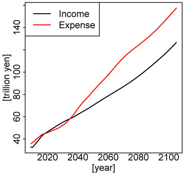
Figure 8. Estimations of the income and the expense of the Japanese welfare pensions. The black and red lines represent estimations of their income and the expense respectively.
4.1, we set  to obtain the stationary
  and
and . We are unable to expect the stationary
  because
  explicitly depends on
 . We assume that our wealth coincide with the benchmark at the initial time:
 . Then we simulate
  paths of
  on
on  according to Equations (1)-(3) using a standard Euler-Maruyama scheme with time-step
  which means that we can rearrange our portfolio every quarter. Results of the simulations are as follows.
We are able to argue that our strategy hedges the shortfall well since Figure 9 suggests that , the averaged hedging error, is approximately 3% of
 , the shortfall, in every quarter.
Figure 10 displays the asset allocation on the sample path described in Figure 11. In the same manner as in the case of the artificial liabilities discussed in Section 4.1, our optimal portfolio is dominated by the money market account, the domestic bond and the foreign stock. However the proportion of the domestic bond and the foreign stock is much higher. We can understand this phenomenon intuitively: since the shortfall increases more rapid than that discussed in Section 4.1, the hedging portfolio is rearranged to become more profitable. The practical suggestion from this fact is that we have to take a risk to track the increasing liability and this is
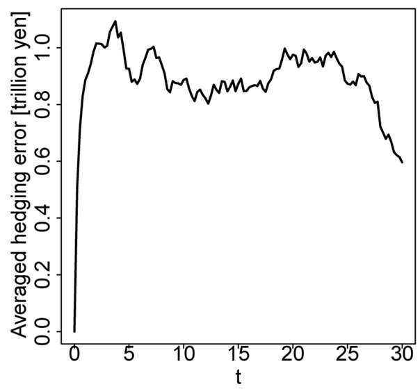
Figure 9. Averaged hedging error .
.
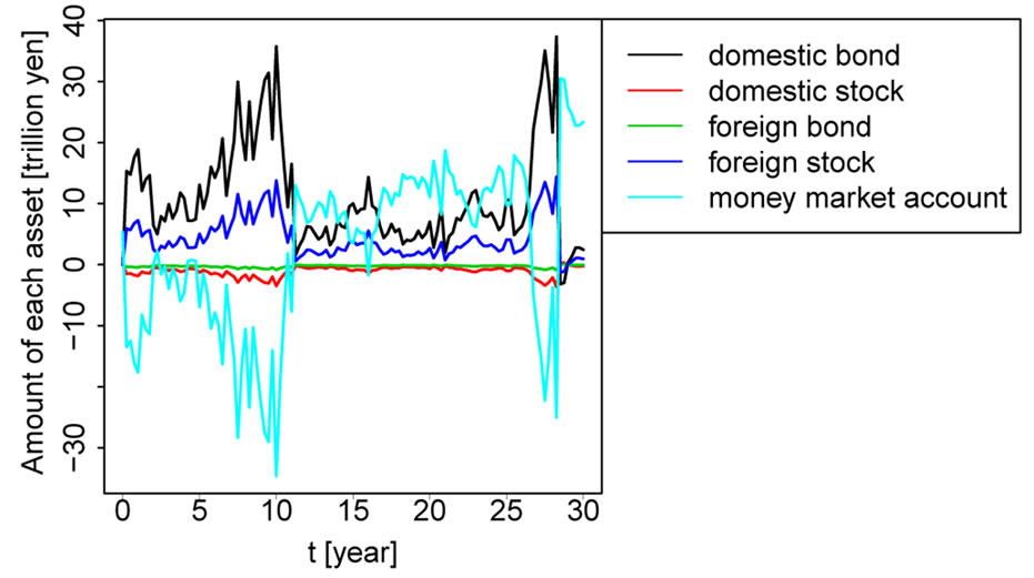
Figure 10. An amount of each asset on the sample path described in Figure 11. The black, red, green, blue and light blue lines represent the amount of a domestic bond, a domestic stock, a foreign bond, a foreign stock and money market account respectively.
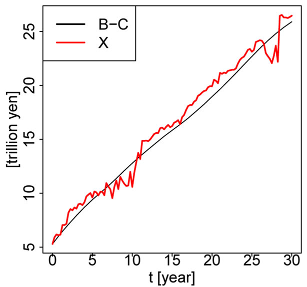
Figure 11. A sample path of  and
and . The black and red lines represent
  and
and  respectively.
quite natural.
5. Summary
We have proposed a long term portfolio management method which takes into account a liability. The LQG control approach allows us to construct a more suitable long term portfolio strategy than myopic one obtained by the single time period mean variance approach in the sense that we are able to change the strategy at any time. Our optimal portfolio strategy hedges the liability by directly tracking the benchmark process which represents the liability. The strategy is evaluated by the mean square error from the benchmark and hence it is intuitive. Two numerical simulations are served: the former one suggests the situation that our portfolio strategy works well; the latter one provides the result with the empirical data published by Japanese organizations. The result demonstrates that our portfolio strategy is able to hedge the liability, the shortfall of the income of the Japanese welfare pension, over three decades.
This study leaves ample scope for further research. Since our criterion is the mean square error, our portfolio strategy inhibits that our wealth exceeds a liability. This is the similar problem with the traditional mean variance approach. One of approaches to avoid it is that we extend criterion which is able to hedge only the case that our wealth goes under the liability. Then we again face the problem of computability as mentioned in the introductory section.
6. Acknowledgements
This work is partially supported by a collaboration research project with the Government Pension Investment Fund in Japan in 2011-2012.
REFERENCES
- The CPP Investment Board, 2013. http://www.cppib.ca/Investments/Total_Portfolio_View/
- W. H. Fleming and R. W. Rishel, “Deterministic and Stochastic Optimal Control,” Springer-Verlag, New York, 1975. doi:10.1007/978-1-4612-6380-7
- G. Deelstra, M. Grasselli and P.-F. Koehl, “Optimal Investment Strategies in the Presence of a Minimum Guarantee,” Insurance: Mathematics and Economics, Vol. 33, No. 1, 2003, pp. 189-207. doi:10.1016/S0167-6687(03)00153-7
- M. Di Giacinto, S. Federico and F. Gozzi, “Pension Funds with a Minimum Guarantee: A Stochastic Control Approach,” Finance and Stochastics, Vol. 15, No. 2, 2010, pp. 297-342. doi:10.1007/s00780-010-0127-7
- F. Menoncin and O. Scaillet, “Optimal Asset Management for Pension Funds,” Managerial Finance, Vol. 32, No. 4, 2006, pp. 347. doi:10.1108/03074350610652260
- R. Gerrard, B. Højgaard and E. Vigna, “Choosing the Optimal Annuitization Time Postretirement,” Quantitative Finance, Vol. 12, No. 7, 2012, pp. 1143-1159. doi:10.1080/14697680903358248
- The Government Pension Investment Fund in Japan, 2013. http://www.gpif.go.jp/operation/committee/pdf/h191001_appendix_05.pdf
- The Japanese Ministry of Health, Labour and Welfare, 2013. http://www.mhlw.go.jp/seisakunitsuite/bunya/nenkin/nenkin/zaisei-kensyo/index.html
Appendix
Proof of Theorem 1
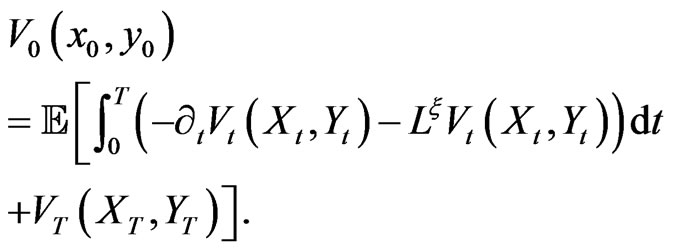
The value function corresponding to our problem (5) is defined by

Hence the corresponding Hamilton-Jacobi-Bellman (HJB) equation is given by
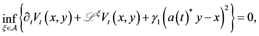 (13)
(13)
with terminal condition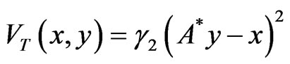 ,
,
 , where
  is partial differential operator with respect to
  and
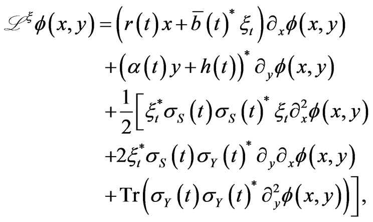
and  is the infinitesimal generator of the process
 :
:
 (i)
(i)
for . Here
  and
and  are the
  -th order partial differential operators with respect to
  and
and . As
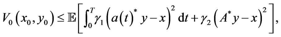
. As  is positive definite, the infimum of (13) is attained at
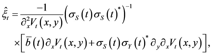
and hence (13) can be written as
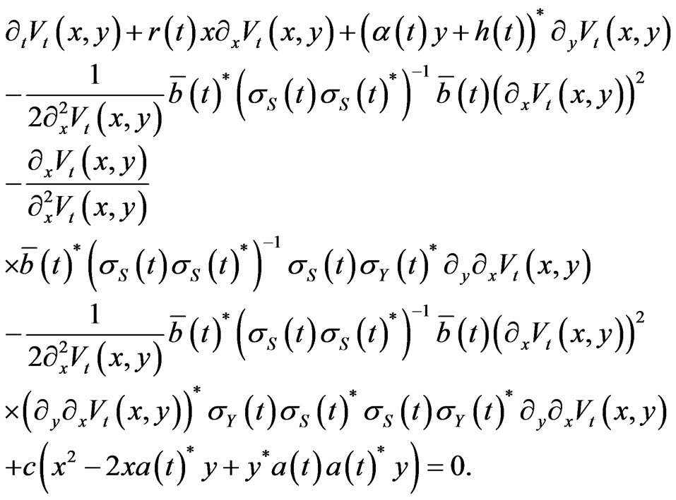
(ii)
Let us try a value function of the form
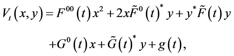
where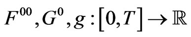 ,
,  and
and
 is a time-dependant symmetric matrix. It is straightforward to see that
 (14)
(14)
 (15)
(15)
 (16)
(16)
 (17)
(17)
 (18)
(18)
 (19)
(19)
and then the associated candidate strategy is represented by
 (iii)
(iii)
Since (14) and (15) are linear ODEs, they have unique solutions on . The existence of unique
  suggests that (16) and (17) are linear ODEs. Hence (16) and (17) also have unique solutions on
 . In the same manner, the existence of unique solutions of (18) and (19) are guaranteed. Therefore
  since
since  and
and  in
in .
.
We now start the verification, i.e., we show that
 ,
,  and
and . To this end, we introduce a sequence of stopping times
  s.t.
s.t.
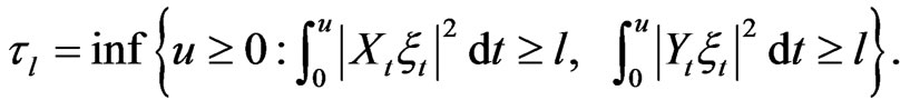
Applying the Ito formula to  and taking expectation, we have
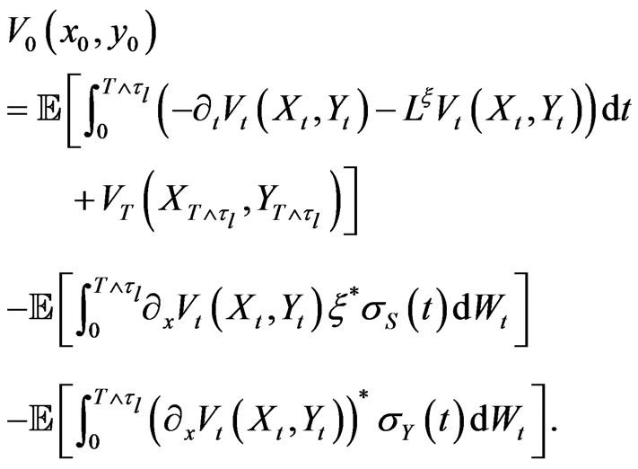 (iv)
(iv)
As  and
and  are in
  and
and ,
,  ,
,  and
and  are continuous functions on
 , the last term vanishes:
 (v)
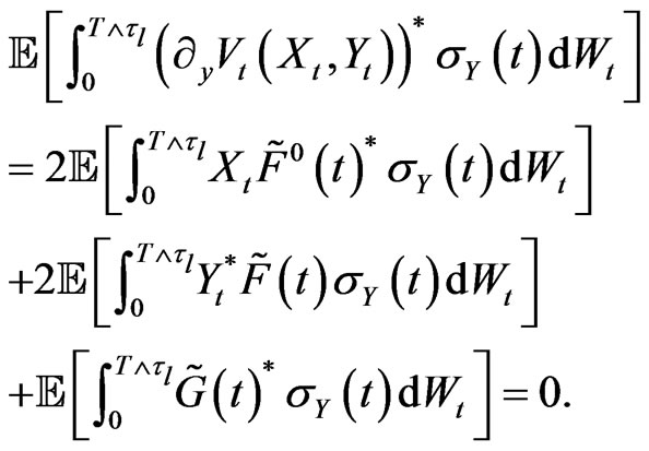
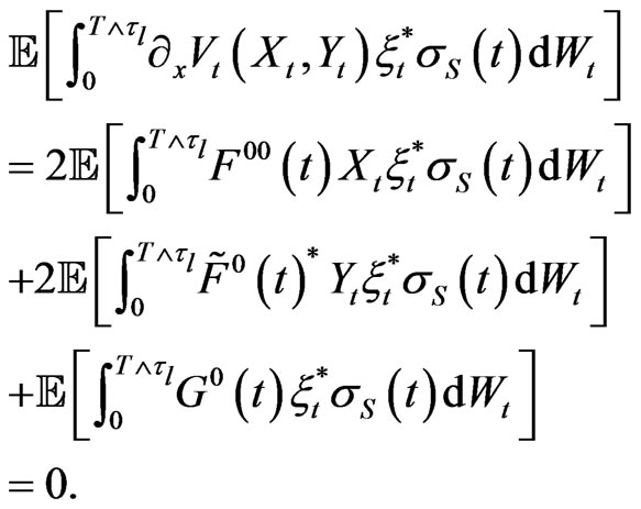
(v)
By the definition of , the continuity of the functions
 ,
,  and
and , and the fact that
 , the remaining stochastic integral term also vanishes:
 (vi)
(vi)
Since  when
when  goes to infinity, we get
 (vii)
(vii)
By the HJB Equation (13) and its terminal condition, we obtain
which means that ,
, . In the same manner we find that
  and then the claim is established.