Open Journal of Statistics
Vol.08 No.05(2018), Article ID:87611,9 pages
10.4236/ojs.2018.85055
An Examination of Male and Female Monthly Employment Rates over Time in Canada and the United States Using Hidden Markov Probability Models
William H. Laverty1, Ivan W. Kelly2*
1Department of Mathematics and Statistics, University of Saskatchewan, Saskatoon, Canada
2Professor Emeritus, University of Saskatchewan, Saskatoon, Canada

Copyright © 2018 by authors and Scientific Research Publishing Inc.
This work is licensed under the Creative Commons Attribution International License (CC BY 4.0).
http://creativecommons.org/licenses/by/4.0/


Received: August 23, 2018; Accepted: September 26, 2018; Published: September 29, 2018
ABSTRACT
In this paper, we will illustrate the use and power of Hidden Markov models in analyzing multivariate data over time. The data used in this study was obtained from the Organization for Economic Co-operation and Development (OECD. Stat database url: https://stats.oecd.org/) and encompassed monthly data on the employment rate of males and females in Canada and the United States (aged 15 years and over; seasonally adjusted from January 1995 to July 2018). Two different underlying patterns of trends in employment over the 23 years observation period were uncovered.
Keywords:
Employment Trends, Hidden Markov Models, Multivariate Data, Canada, United States

1. Introduction
The literature on economic and employment data is extensive and addresses specific issues of interest to government policy, educational, and business concerns. The Organization for Economic Co-operation and Development (OECD) provides data on well-being and economic data from 36 countries (URL: https://stats.oecd.org/) [1] . In this article, we compare both male and female Canadian and American (USA) employment rates over a 23-year period. The purpose of the study will be to utilize the statistical procedure of Hidden Markov Models to uncover underlying trends and changes in monthly employment rates in the two countries.
Traditionally, time series analysis has been used to analyze employment and related data over time. Many of the time series models (Autoregressive Moving Average (ARMA), Autoregressive Integrated Moving Average (ARIMA), etc.) assume that the mechanism driving the models is constant over time. If the data is observed over a long period of time, it is very likely that there are changing underlying states that generate data from different distinct models. In this instance, the appropriate model of the data is the Hidden Markov Model (HMM). Hidden Markov Models (HMMs) are a widely used collection of statistical models. These models are applicable when studying a process that goes through a sequence of states. These states are unseen (hidden) but what is observed is data from each state. This means that the HMMs have potentially very wide applications across a large variety of fields, including physical and psychological development in human beings as well as the examination of physiological changes in medicine (HMMs have been used to model heart rate variability [2] ). In our own research, we have modeled residuals in regression [3] [4] . In the economic field, HMMs have been used to model financial data [5] , stock market performance ( [6] , forthcoming), and predicting foreign exchange rates [7] and so on.
In this paper, we will illustrate the use and power of Hidden Markov Models in analyzing multivariate data over time. The customized data examined here encompasses monthly data on the employment rate of males and females in Canada and the United States (aged 15 years and over; seasonally adjusted from January 1995 to July 2018.) The 23-year period was considered sufficient to uncover any underlying employment trends of interest. For our purposes, and for simplification, we did not include variables, such as age, socio-economic status, part-time vs. full-time employment, geographical location, etc.
2. Method
2.1. Hidden Markov Mathematical Model
A hidden Markov model consists of a sequence of states X1, X2, …, XT, together with a sequence of observations Y1, Y2, …, YT. The total number of states (possible values of each Xi) we will assume is a finite number, m. In this case the states can be represented by the integers 1, 2, ..., m. The states are not observed. The observations Y1, Y2, …, YT are observed and could be vectors of dimension k. The distribution of Yt depends on the state Xt, the state the Markov process is in at time t. In this paper we are assuming that that the distribution of Yt if Xt = i (i = 1, 2, … m) is the Multivariate Normal distribution with mean vector and covariance matrix Si.
The parameters of the hidden Markov model are the initial state probabilities,
and the transition probability matrix Γ = (γij). This is an m x m matrix, with element γij being the probability of a transition into state j starting from state i.
i.e.
,
where t denotes time. These two choices allow a sequence of states (known also as the Markov chain) X1, X2, …, XT constituting the hidden part of a hidden Markov model.
When the Markov chain is in state i, at time t, it emits an observed signal Yt, which is either a discrete or a continuous random variable (or random vector) with distribution conditional on the current state i.
In the discrete case
where pi is probability mass function with parameters θi. In the continuous case the conditional density of Yt = y given Xt = i is fi(y; θi)
In this paper we will assume that fi(y; θi) is the Multivariate Normal distribution with mean vector and covariance matrix Si.
There are several statistical questions associated with Hidden Markov models:
1) Given the observed data, what are the estimates of the parameters of model.
a) The initial state probabilities.
b) The state transition probabilities.
c) The parameters of the distribution of the observation vectors Yt when the Hidden Markov chain is in state i. ( and Si.)
2) Given the observed data, and the estimated parameters of model, what are the sequence of unknown states, X1, X2, X3, …, XT that generated the data.
2.2. Subjects
The data used in this study was obtained from the Organization for Economic Co-operation and Development (OECD) and consisted of monthly employment rates on both males and females (aged 15 years and over; seasonally adjusted) over a 23.5 year period (January 1995 to July 2018).
2.3. Measure
The measure used in this study was monthly rate of employment for each of Canadian and USA males and females as reported in the OECD database.
3. Statistical Analysis
The initial analysis of the data consisted of graphs of the raw data and changes in the employment rate for all four groups over the time period under consideration. The estimation of the parameters of a Hidden Markov model (HMM) and computation of posterior probabilities of states were subsequently determined. A Hidden Markov statistical model was used to uncover hidden states in the data and the mean vectors and standard deviation for the states was determined. A correlation matrix and principal components were calculated for each state uncovered. The estimation of the parameters of the Hidden Markov model (HMM) and computation of posterior probabilities of states was achieved using the R program, depmixS4.
4. Results
The data consisting of male and female employment rates over the 23 year period were graphed to give an overall picture.
All graphs indicate periods of both increasing and decreasing trends in employment rates for males and females in both countries. The following Graphs (Figure 1) are the changes in monthly employment rates for males and females in both countries.
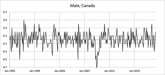
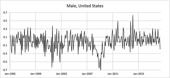
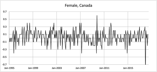
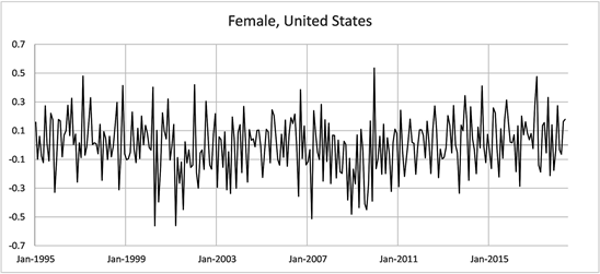
Figure 1. Changes in employment Rate Aged 15 - 64, January 1995-June 2018.
These graphs show volatility in the month to month changes in monthly employment rates. Without further analysis it is difficult to assess whether the central values of the monthly changes in employment rates are nonzero (positive or negative) during particular periods of time. We will now apply the use of HMM models to uncover hidden states in trends that are not visually evident in the above graphical data.
The Estimation of the Parameters of a Hidden Markov Model (HMM) and Computation of Posterior Probabilities of States
The data that was analyzed was the monthly changes in employment rates of males and females of the two countries over the observed period. Our analysis indicated that two underlying states were uncovered.
From Table 1, the Matix transition probabilities determine the expected duration of the uncovered states: the expected duration spent in state 1 is 1/(1 − 0.893) = 9.35 months while the expected duration spent in state 2 is 1/(1 − 0.975) = 40.00 months. In other words, once the process enters state 1 the average length of time it remains in that state is 9.35 months (and 40 months for state 2).
One can note (Table 2) that for both underlying states, the standard deviation of both males and females monthly employment rates is large relative to the mean monthly change. This is indicative of the volatility observed in the previous graphs (Figure 1) of monthly employment changes. In state 1, the means of monthly changes are negative (with the exception of Canadian females) indicating the employment rate is decreasing. The mean of zero for Canadian females is indicative of a random walk. In state 2, the mean monthly changes are all positive, indicating increasing employment for both males and females in both countries.
Table 3 and Table 4: Correlation Matrix and Principal Components for state 1.
Principal components are a technique for understanding complex correlation structures. The first principal component is a linear combination of the observations that accounts for the maximum percentage of variance in the observations. Subsequent principal components (PCs) are independent of the previous PCs and account for the maximum variance in the observations that has not been accounted by the previous PCs. The first principal component account for all of the variability of monthly employment changes during state 1. The first principal component can be interpreted as increasing or decreasing numbers in the employment changes for all four groups simultaneously. The loadings on the next three principal components result in groupings based on negative or positive sign. The second principal component is a comparison between Canadian and American employment changes when in the first state and account for 23.4% of the total variation in the rate changes. It will be noted that American increase in employment rate occurs with Canadian decrease. The third principal component is a comparison heavily weighted on Canadian males compared with the other three groups. The fourth principal component associated with state 1 is an effect of gender restricted to the USA, notably American females versus American males.
Table 5 and Table 6: Correlation Matrix and Principal Components for state 2.
The first four principal components account for approximately the same contribution to variability within monthly changes during state 2. This finding usually occurs when the variables are independent. Table 5 supports this with the low correlations among pairs of variables. In such a situation the principal components do not provide much information.
In a Hidden Markov model one is interested in determining the underlying hidden state at each point in time suggested by the data. The following graph (Figure 2) plots the posterior probability of being in state 1 (the probability of being state 2 is just 1-the probability of being in state 1).
Looking again at Figure 3, we can see roughly the two different states: HMM state 1 employment rates decreasing in three categories (American Males, American Females, Canadian Males). In state 2 employment rates are increasing in all four groups. Figure 3 also illustrates the properties that the average length of time remaining in state 1 to be 9.35 months (and 40.00 months for state 2), which is implied by the transition matrix (Table 1).

Table 1. Transition matrix of state transitions, assuming only two states.
Table 2. Mean vectors and Standard deviations for the two states.
Table 3. Correlation matrix.
Table 4. Principal components.
Table 5. Correlation matrix.
Table 6. Principal components.
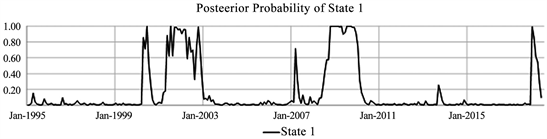
Figure 2. Posterior probability of State 1.
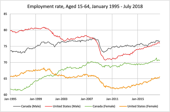
Figure 3. Employment rates for Canada and the United States for males and females in the age group 15 - 64.
5. Conclusions
This example utilizing employment data illustrates the usefulness of the Hidden Markov Model in studying a multiple dimensional process that is changing over time. From this analysis, we see that over a 23-year period (1995-2018), the trends in Canadian and United States employment rates do not follow a single pattern (or single state). The HMM analysis has shown at least two underlying patterns in employment trends. This would be missed by traditional time series analysis which assumes a common state over time. In the first state (shorter lasting), the number of employees in both Canada and the United States is decreasing (with the exception of Canadian women). In the second state, longer in duration, there are small monthly increases in all four groups. In employment data, there are states of high and low volatility. The HMM model provides more precise measurements of how long employment data stay in uncovered states. The conditions that generate observations over time do not stay constant for long periods of time. The underlying conditions (states) change if observed for long periods of time. The HMM takes this into account.
In our analysis, we assumed independence between monthly observation vectors while the process was in a constant state. This assumption could be dropped and assume autocorrelation within states. In this latter case, one would apply an Autoregressive Hidden Markov analysis (e.g. see [8] ) of the data. A more refined analysis might also reveal such patterns exhibit differently according to age, socioeconomic status, ethnicity, etc. or interactions among these variables.
A similar analysis could be conducted over a variety of fields where data is collected over time. The important requirement is not the absolute length of time (23 years in this example) but the frequency of observations and frequency of state changes. For example, the classical example of the use of Hidden Markov models was in speech recognition (Rabiner, 1989) where the length of data sequences was a few seconds. With the increase in the ability to collect longitudinal health and social data, these provide fruitful areas for the application of these techniques.
Conflicts of Interest
The authors declare no conflicts of interest regarding the publication of this paper.
Cite this paper
Laverty, W.H. and Kelly, I.W. (2018) An Examination of Male and Female Monthly Employment Rates over Time in Canada and the United States Using Hidden Markov Probability Models. Open Journal of Statistics, 8, 837-845. https://doi.org/10.4236/ojs.2018.85055
References
- 1. The Organization for Economic Co-Operation and Development (OECD). https://stats.oecd.org/
- 2. Walker II, M. (2011) Hidden Markov Models for Heart Rate Variability with Biometric Applications. All Theses and Dissertations (ETDs).
- 3. Laverty, W.H., Miket, M.J. and Kelly, I.W. (2002) Application of Hidden Markov Models on Residuals: An Example Using Canadian Traffic Accident Data. Perceptual and Motor Skills, 94, 1151-1156. https://doi.org/10.2466/pms.2002.94.3c.1151
- 4. Laverty, W.H., Miket, M.J. and Kelly, I.W. (2002) Examination of Residuals to Vancouver Crisis Call Data by Using Hidden Markov Models. Perceptual and Motor Skills, 94, 548-550. https://doi.org/10.2466/pms.2002.94.2.548
- 5. Bhar, R. and Hamori, S. (2004) Hidden Markov Models: Applications to Financial Economics. Springer, Switzerland.
- 6. Lihn, S. (Forthcoming) Hidden Markov Model for Financial Time Series and Its Application to S & P 500 Index. Quantitative Finance.
- 7. Nootyaskool, S. and Choengtong, W. (2014) Hidden Markov Model Prediction of Foreign Exchange Rate. International Symposium on Communications and Information Technology, Incheon, 24-26 September 2014.
- 8. Xuan, T. (2004) Autoregressive Hidden Markov Model with Application in an El Nino Study. MSc. Thesis, University of Saskatchewan, Saskatoon.