Received 18 December 2015; accepted 20 February 2016; published 23 February 2016

ABSTRACT

We present Bayes estimators, highest posterior density (HPD) intervals, and maximum likelihood estimators (MLEs), for the Maxwell failure distribution based on Type II censored data, i.e. using the first r lifetimes from a group of n components under test. Reliability/Hazard function estimates, Bayes predictive distributions and highest posterior density prediction intervals for a future observation are also considered. Two data examples and a Monte Carlo simulation study are used to illustrate the results and to compare the performances of the different methods.

Keywords:

Bayes Estimator, HPD Interval, Maxwell Distribution, MLE, Prediction, Reliability Function

1. Introduction

The prediction problems of lifetime models are very important and have been studied, among others by Aitchi- son & Dunsmore (1975) [1] , Chhikara & Guttman (1982) [2] , Dunsmore (1974) [3] , Evans & Nigm (1980) [4] , Howlader(1985) [5] , Lawless (1977) [6] and Likes(1974) [7] .

Tyagi and Bhattacharya (1989a, b) [8] [9] considered the Maxwell distribution as a lifetime model and obtained the Bayes and the minimum variance unbiased estimators of the Maxwell parameter and its reliability function. Howlader and Hossain (1998) [10] also considered the Maxwell distribution and provided Bayes estimates for the parameter θ, its associated reliability function, and highest posterior density intervals (HPD) for θ.

The purpose of this paper is to derive maximum likelihood estimators (or estimators that maximize the likelihood function), Bayes estimators in terms of the mean of the posterior distribution, and highest posterior density intervals for θ (which are intervals with a posterior probability of and minimum length), the reliability function and the hazard function based on Type II censored data. In addition, we present Bayes predictive estimators based on predictive means and HPD prediction intervals for a future ob- servation. When sampling is expensive and time consuming, the Type II censoring scheme can be used to save on the cost of the experiment and the data collection time. From a Bayesian perspective, estimation of lifetime models under censoring has been investigated by many authors (Balakrishnan (1990) [11] , Bekker and Roux (2005) [12] , Chaturvedi and Rani (1998) [13] ).

The Maxwell probability density function (pdf) and cumulative distribution function (cdf), are respectively given by:

(1)

and

where is the incomplete Gamma function defined by

A result we will use in the developments of this paper is the following. If distribution,

follows a. The pdf of Y is given by

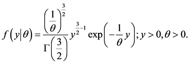(2)

From a Bayesian perspective, in this study, we consider an asymptotically locally invariant prior, , proposed by Hartigan (1964) [14] which is derived from distributions satisfying:

where

and and.

For the pdf (1), it can be shown that (Howlader and Hossain (1998) [10] )

(3)

In addition, we consider Jeffreys prior given by

where is the expected Fisher’s information. For the pdf (1) it can can be shown that

(4)

In Section 2, we describe the procedure for estimating the parameter θ, the reliability function, and the hazard function. In Section 3, we discuss how HPD intervals for θ and are obtained. In Section 4, we describe how Bayes predictive estimators and highest posterior density prediction intervals for a future observation are produced. Finally, Sections 5 and 6 provide results for two data examples and a simul- ation study. The conclusions are presented in Section 7.

2. Estimation of θ, h(t;θ), and R(t;θ)

We assume a group of n components have lifetimes which follow a Maxwell distribution. The failure times are recorded as they occur until a fixed (known) number r of components have failed. As it is quite common in life testing situations, (e.g., destructive tests, high cost of testing an item, etc.) only the first r lifetimes in a sample of n units can be obtained. Let where is the time of the ith component to fail. Since the remaining components have not yet failed and thus, they have lifetimes greater than, the maxi- mum of the observed sample. This is what we refer to as Type II censoring. Instead of x we work with

and. Since the lifetimes in x follow a Maxwell distribution,

for. For observations when,

, i.e., a distribution truncated to the interval.

Therefore, the likelihood function for θ in terms of y can be written as,

(5)

where is a pdf and is the CDF of a evaluated at.

Furthermore,

(6)

and the log-likelihood is equal, except for a constant, to

(7)

The maximum likelihood estimator (MLE) of θ, , is found by numerical maximization of the log- likelihood. Relying on asymptotic normality properties of the MLE under Type II censoring as in Kong and Fei (1996) [15] , an approximate confidence interval for θ can be obtained from,

where is Fisher’s information evaluated at and is the

quantile of a distribution.

By the invariance property of MLE’s, we get that the MLE of the reliability function, is

(8)

Also, the MLE for the failure rate or hazard function, is

(9)

Bayes Estimation

Combining the likelihood function and the prior, the posterior density of is given by the expression,

(10)

A squared error loss is appropriate when decisions become gradually more damaging for larger errors. The Bayes estimator of under this loss function is the posterior expectation of,

(11)

In general, this expected value does not have a closed form solution. We rely on MCMC calculations to approximate. For the case of the Maxwell distribution, transformed into a Gamma model, MCMC can be done with the Openbugs software as in Lunn et al. (2012) [16] . If is a MCMC sample from, after a burn-in period and convergence has been checked,

(12)

The Bayes estimates of (reliability function) and (failure rate function) do not have a closed form and so we consider numerical integration to approximate its values. The approximate Bayes esti- mates of and, under a squared loss function with a MCMC sample are,

(13)

and

(14)

By graphing posterior realizations of and as a function of t, we an provide an uncertainty band for these functions in addition to the point estimates and.

3. Intervals for θ and R(t,θ)

A credible interval for θ can be obtained by taking our sample and finding the and sample quantiles, and respectively. interval for θ is given by. This interval approximately satisfies the condition that

(15)

Analogously, for the reliability function, we transform our MCMC samples for θ and obtain a

sample for of values. The sample quantiles and based

on these values provide a interval of. In a similar way, we can produce credible intervals for the hazard function.

It is not automatic to compute a highest posterior density (HPD) interval from a Monte Carlo sample specially if the posterior is far from symmetric or multimodal. However, we use the method in Liu, Gelman and Zheng (2013) [17] , to obtain HPD intervals from a MCMC sample based on a numerical approximation to HPD intervals integrated in the SPIn R-package. We use this method to compute HPD intervals for parameters or predictions for this paper.

4. Bayes Predictive Estimator and Intervals

Let z be a future observation which has already survived. Given the data x, the conditional joint p.d.f of z and θ is

(16)

and takes into account censoring. To produce a Monte Carlo sample of the predictive distribution, we can do it in two steps typically referred to as the Method of Composition:

1. Sample.

2. Sample.

3. Repeat steps (1) and (2) M times where M represent a fixed number of MCMC samples.

This procedure provides a sample, , of values that correspond to the predictive distribution. The Bayes estimator of z under squared error loss function can be approximated as

(17)

A predictive interval for z can be found by making and, the and

sample quantiles of. The HPD interval can be computed with the SPIn method. In our numerical examples, we found that the SPIn method could provide some different results depending on how we thin the MCMC sample and select the M value. At this point, it is worth mentioning that Bayesian estimation and prediction of the two-parameter Gamma distribution has been considered in Pradhan and Kundu (2011) [18] . However this other paper does not explicitly address estimation and prediction under type II censoring as we propose here.

5. Numerical Examples Using Real Data Sets

5.1. Example 1: National Radio Astronomy Observatory Data Set

The following data represent noise levels in cryogenic microwave receivers and were obtained from Darrell Hicks at the National Radio Astronomy Observatory, Socorro, NM. We arranged the observations in ascending order and dropped the last 11 data points to induce censoring, which leads to a situation with n = 86 and r = 75. After transforming the data with x²,. The values of are: 1.69, 2.56, 2.89, 3.24, 4.00, 4.00, 4.00, 4.84, 4.84, 5.29, 5.29, 5.29, 5.76, 5.76, 6.25, 6.25, 6.76, 6.76, 6.76, 7.29, 7.29, 7.84, 7.84, 8.41, 8.41, 8.41, 8.41, 8.41, 8.41, 9.00, 9.00, 10.24, 10.89, 10.89, 11.56, 11.56, 11.56, 11.56, 11.56, 12.25, 12.25, 12.96,12.96,13.69, 14.44, 14.44, 14.44, 14.44, 15.21, 16.00, 16.81, 17.64, 17.64, 17.64, 17.64, 17.64, 18.49, 20.25, 21.16, 25.00, 33.64, 36.00, 36.00, 37.21, 38.44, 42.25, 42.25, 43.56, 47.61, 57.76, 62.41, 68.89, 72.25, 81.00, 86.49.

The MLE of θ obtained numerically with a Nelder-Mead, Quasi-Newton algorithm (in 100-th units) is = 20.17. A graph of the MLEs, and is shown in Figure 1. After a burn-in of 1000 MCMC iterations, the posterior mean estimate of θ based on 5000 additional samples results in. MCMC convergence is reached after only a few iterations and was checked with time series plots of the iterations (trace plots) and autocorrelation plots. Based on our sample and as described in Section 3, a 95% credible interval for θ is (16.98, 24.36). For comparison and relying on MLE asymptotic theory, we also computed an approximate 95% confidence interval for θ which resulted in the interval (16.51, 23.58). For this calculation, the expected Fisher’s information was approximated with the observed information obtained from the Hessian calculation (matrix of second derivatives) resulting from the Nelder-Mead, Quasi-Newton method.

In Figure 2 (top), we show a histogram of the posterior samples of θ along with the density representation of its posterior distribution. Figure 3 presents the posterior mean (in solid black line) and 200 posterior samples for the reliability function (top) and the hazard function (bottom). From this figure we observe that when t approaches the value of 10, the reliability function values are close to zero. For the hazard function, the failure rates are monotonically increasing as a function of t. Based on the sampling scheme described in Section 4, Figure 2 (bottom) also shows samples of the posterior predictive for a future observation z taking into account censoring and its approximate density function. The predictive mean for a future observation is 10.40 and a 95% predictive interval for a future observation is (9.63, 13.10). These values remain essentially the same using either Jeffrey’s prior or Hartigan’s prior on θ. The results obtained with the SPIn R-package to compute

HPD intervals from our MCMC samples are as follows. The HPD interval for θ is (16.78278, 24.48906) which is not very different compared to an interval based on the 0.25 and 0.975 sample quantiles. The HPD for the predictive distribution of a future z observation is (9.36, 12.82) which also remains similar to the one reported with 0.25, 0.975 sample quantiles. In Table 1, we report 95% HPD intervals for future observations for different levels of censoring. It should be noted that the width of the interval increases as the level of censoring increases. On the other hand, the predictive interval without censoring captures all the variability that is present in the full data set.

5.2. Example 2: Burning Velocity of Different Chemical Materials

We now use the Kazmi et al. (2012) [19] data set that consists of 55 observations related to the burning velocity of different chemical materials. The burning velocity is the velocity of a laminar flame under stated conditions of composition, temperature, and pressure. It decreases with increasing inhibitor concentration and can be

determined by analyzing the pressure profiles in the spherical vessel and checked by direct observation of flame propagation. The data related to the burning velocity (cm/sec) of different chemical materials is given below: 68, 61, 64, 55, 51, 68, 44, 82, 60, 89, 61, 54, 166, 66, 50, 87, 48, 42, 58, 46, 67, 46, 46, 44, 48, 56, 47, 54, 47, 80, 38, 108, 46, 40, 44, 312, 41, 31, 40, 41, 40, 56, 45, 43, 46, 46, 46, 46, 52, 58, 82, 71, 48, 39, 41. The source of the above explained data related to the burning velocity of different chemical materials for the year 2005 is available from http://www.cheresources.com/mists.pdf. In this paper, and to compute our estimates, we consider the units of burning velocity as m/sec.

In Table 2, we report HPD intervals for θ corresponding to this data set under 3 different priors: Hartigan’s, Jeffreys’ and a Gamma(1,1) prior which is an Exponential distribution of decay parameter equal to one. The

lengths of the HPD intervals for θ under Hartigan prior are slightly shorter compared to the intervals obtained with Jeffreys’ and Gamma priors for both censoring times considered.

In addition, we also computed the approximate 95% confidence interval for θ with the MLE asymptotic approximation to the Normal distribution as described in Section 2. For a censoring time of 64(0.64), the interval is (0.1706, 0.2790) and for a censoring time of 68 (0.68), the interval is (0.1681, 0.2697). Again, the expected Fisher’s information was approximated with the observed Fisher’s information at the MLE. In contrast to the NRAO data set example, the HPD intervals provide different results compared to a MLE approximation that relies in asymptotic normality.

6. Monte Carlo Simulation Studies

In order to assess the performance of the estimation and prediction approaches proposed in this paper, we perform a Monte Carlo simulation study based on 5000 simulated data samples of sizes n = 15, 25, 35, 50 and 100 with 10% and 30% censoring respectively. For each of our simulated data samples, we computed the Bayes estimates using a squared error loss function after a burn-in of 500 MCMC iterations. For different values of t and using the above mentioned sample sizes, we computed the average Bayes estimates, and, as in Section 2. The main results are presented in Table 3 and Table 4. The true value of θ for the simulation was selected equal to 20.5. The “true” reliabilities for this θ value for t = 0.5, 2.5, 5.0 and 7.5, are respectively: 0.9990, 0.8942, 0.4864 and 0.1394 and the ‘true’ hazard function values are respectively: 0.0060, 0.1253, 0.3691 and 0.6312. We have done some other simulations using different values of θ and the pattern of the numerical results remain similar to those reported here.

Furthermore, for a second simulation based on 5000 samples and for various values of θ, in Figure 4, we show Mean Square Error (MSE) curves for a posterior θ computed under Hartigan, Jeffreys’ prior and the MLE method respectively. For each data simulation and parameter, we produce an estimate through the 3 approaches and compute a square error difference between the true parameter value and the estimated value. An average was obtained across simulation and graphed as a function of θ. The results show that as θ gets larger, the MSE values are increasing. We also note that except for the first case, where no censoring was considered, the MSE curves under Hartigan’s prior are lower than those obtained with Jeffreys or MLE. Various values of n and r were considered in this study and defined the four panels shows in Figure 4. The top left panel refers to a case where there is no censoring N = 86, r = 86, the top right panel is for N = 86, r = 81. For the bottom panel, we have N = 86, r = 70 (right panel) and N = 86, r = 65 for the left panel. We notice that the differences between the curves corresponding to each prior are more marked when the censoring level increases.

7. Conclusions

The main contribution of this paper is to obtain the parameter estimates for the Maxwell failure distribution under Type II censoring via the Gamma distribution, using Bayesian estimation under different priors and compared it with Maximum Likelihood Estimation (MLE). MLE can be thought as the maximum of the posterior distribution under an unrestricted uniform prior. We observe from Table 1 (NRAO data example) that the length of the 95% HPD prediction intervals for future observations increases as the percentage of censoring increases. The width of the HPD intervals under censoring is shorter as compared to non censored data. It can be noted from Table 2 (Burning velocity data example) that at censoring t = 64 and censoring t = 68, the HPD intervals for θ under Hartigan’s prior are slightly shorter than for both Gamma and Jeffreys priors. From Table 3 (simulation study), it can be observed that the values of the Bayes estimates are larger for all samples

sizes and for small values of t. When t increases the values of decreases for all sample sizes. The same pattern is observed for Table 4 (simulation) when censoring is set equal to 30%. The values of increase when t increases for all the sample sizes studied for both 10% and 30% censoring. For the estimation of the parameter θ, with Type II censoring, the MSE calculations of Figure 4 show that Hartigan’s prior has a better performance than Jefferys’ prior and MLE. This is true for all of the values of the parameter θ that are studied and all values of n and r considered but it is more noticeable for cases where there is more censoring.

For estimating the parameter θ of the Maxwell distribution under Type II censoring, it appears to be clear from all our numerical results that Bayes estimation is appropriate or in some cases, superior than MLE, but with the MLE method as a good competitor. In the second data example for which the sample size n = 55, an approximate 95% confidence interval for θ provides a result that is different to HPD intervals. A limitation of our approach is the use of a square data transformation for the Gamma distribution which can pose challenges under the Type II censoring for large numerical data values. The priors considered for comparisons are obtained under the non-censored case, therefore, a similar study can be attempted computing Jeffreys’ and Hartigan’s priors numerically and where the Type II censoring is incorporated into the likelihood function. An Openbugs model that implements the approach described in this manuscript with the Gamma and truncated Gamma distributions, is available by request from the second author.

Acknowledgements

We thank the referee and Editor for their comments and suggestions about our paper. This project was supported

by New Mexico Tech, Socorro, New Mexico, USA and research funds from the College of Arts and Sciences, The University of New Mexico,USA. G. Huerta performed all the computations and simulations applied in this paper. He also proposed the model from a Gamma distribution perspective. The Openbugs model for this paper is available from G. Huerta.

Cite this paper

Anwar M.Hossain,GabrielHuerta, (2016) Bayesian Estimation and Prediction for the Maxwell Failure Distribution Based on Type II Censored Data. Open Journal of Statistics,06,49-60. doi: 10.4236/ojs.2016.61007

References

- 1. Aitchison, J. and Dunsmore, I.R. (1975) Statistical Prediction Analysis. University Press, Cambridge.
http://dx.doi.org/10.1017/CBO9780511569647 - 2. Chhikara, R.S. and Guttman, I. (1982) Prediction Limits for the Inverse Gaussian Distribution. Technometrics, 24, 319-324.
http://dx.doi.org/10.2307/1267827 - 3. Dunsmore, I.R. (1974) The Bayesian Predictive Distribution in Life Testing. Technometrics, 16, 455-466.
http://dx.doi.org/10.1080/00401706.1974.10489216 - 4. Evans, I.G. and Nigm, A.H.M. (1980) Bayesian Prediction for the Left-Truncated Exponential Distribution. Technometrics, 22, 201-204.
http://dx.doi.org/10.1080/00401706.1980.10486135 - 5. Howlader, H.A. (1985) HPD Prediction Intervals for Rayleigh Distribution. IEEE Transactions on Reliability, R-34, 121-123.
- 6. Lawless, J.F. (1977) Prediction Intervals for the Two Parameter Exponential Distribution. Technometrics, 19, 469-472.
http://dx.doi.org/10.1080/00401706.1977.10489587 - 7. Likes, J. (1974) Prediction of s-th ordered observation for the two parameter exponential distribution. Technometrics, 16, 241-244.
http://dx.doi.org/10.1080/00401706.1974.10489180 - 8. Tyagi, R.K. and Battacharya, S.K. (1989a) Bayes Estimation of the Maxwell’s Velocity Distribution Function. Statistica, 4, 563-567.
- 9. Tyagi, R.K. and Battacharya, S.K. (1989b) A Note on the MVU Estimation of the Maxwell’s Failure Distribution. Estadistica, 41, 73-79.
- 10. Howlader, H.A. and Hossain, A.M. (1998) Bayesian Prediction Intervals for Maxwell Parameters. Metron-Interna tional Journal of Statistics, LVI, 97-106.
- 11. Balakrishnan, N. (1990) On the Maximum Likelihood Estimation of the Location and Scale Parameters of Exponential Distribution Based on Multiple Type II Censored Samples. Journal of Applied Statistics, 17, 55-61.
http://dx.doi.org/10.1080/757582647 - 12. Bekker, A. and Roux, J.J. (2005) Reliability Characteristics of the Maxwell Distribution: A Bayes Estimation Study. Communications in Statistics—Theory and Methods, 34, 2169-2178.
http://dx.doi.org/10.1080/STA-200066424 - 13. Chaturvedi, A. and Rani, U. (1998) Classical and Bayesian Reliability Estimation of the Generalized Maxwell Failure Distribution. Statist. Research, 32, 113-120.
- 14. Hartigan, J.A. (1964) Invariant Prior Distributions. The Annals of Mathematical Statistics, 35, 836-845.
http://dx.doi.org/10.1214/aoms/1177703583 - 15. Kong, F. and Fei, H. (1996) Limit Theorems for the Maximum Likelihood Estimate under General Multply Type II Censoring. Annals of the Institute of Statistical Mathematics, 48, 731-755.
http://dx.doi.org/10.1007/BF00052330 - 16. Lunn, D., Jackson, C., Best, N., Thomas, A. and Spiegelhalter, D. (2012) The BUGS Book: A Practical Introduction to Bayesian Analysis. Chapman and Hall/CRC, Bacon Raton.
- 17. Liu, Y., Gelman, A. and Zheng, T. (2013) Simulation-Efficient Shortest Probability intervals. Unpublished Manuscript, 1-22.
http://arxiv.org/pdf/1302.2142.pdf - 18. Pradhan, B. and Kundu, B. (2011) Bayes Estimation and Prediction of the Two-Parameter Gamma Distribution. Journal of Statistical Computation and Simulation, 81, 1187-1198.
http://dx.doi.org/10.1080/00949651003796335 - 19. Kazmi, S.M.A., Aslam, M. and Ali, S. (2012) Preference Prior for the Class of Life-Time Distributions under Different Loss Functions. Pakistan Journal of Statistics, 28, 467-484.