Open Journal of Statistics
Vol.2 No.1(2012), Article ID:17142,13 pages DOI:10.4236/ojs.2012.21007
Comparative Analysis of Group Sequential Designs Tests for Randomized Controlled Clinical Trials: A Model Study on Two-Sided Tests for Comparing Two Treatments
Department of Biostatistics and Medical Informatics, Medical Faculty, Mersin University, Mersin, Turkey
Email: malisungur@yahoo.com
Received July 13, 2011; revised August 18, 2011; accepted August 30, 2011
Keywords: Group Sequential Designs; Group Sequential Test Types; Interim Analysis; Monitoring
ABSTRACT
Clinical trials are usually long term studies and it seems impossible to reach all required subjects at the same time. Performing interim analyses and monitoring results may provide early termination of trial after obtaining significant results. The aim of this study is comparing group sequential tests in respect to advantage of sample size reduction and early termination. In this study, 4 test types used in group sequential designs were compared with fixed sample size design test and each other. Comparisons were done according to two-sided tests for comparing two treatments. In this sense, 1080 models were performed. In models, 2 different Type I errors, 2 different powers, 5 different analysis groups, 6 different effect sizes and 9 different variances selections were considered. All test types increased the maximum sample size in different manner, compared with fixed sample size design. Each test had different critical values to reject H0 hypothesis, at the same type I error rate and number of analyses conditions. Selection of test type used in group sequential designs depends on a few characteristics, as reducing sample size, early termination and detecting minimal effect size. Test performance is highly related with selected Type I error rate, power and number of analyses. In addition to these statistical characteristics, researchers should decide test type with respect to other trial conditions as the issue of trial, reaching subjects easy or not and importance of early termination.
1. Introduction
Clinical trials are designed to detect differences between treatments with a certain power and Type I error rate. Investigators should ensure to design clinical trials that contain adequate statistical power and sample size. It takes a long time to reach required subject number at the same time. Data are accumulated periodically course of the trial. Thus, it may take a few years to enroll enough subjects to meet determined sample size at the beginning of the trial. Particularly, in clinical trials which have death risk or any potential harm this may be more difficult and reaching required sample size may cause more increasing of trial time. Therefore, it is an important interest of investigators substantially to analyze accumulated data in specific intervals and evaluate results. Performing interim analyses and monitoring results may provide early termination of trial after obtaining significant results corresponding superiority, inferiority or equivalency of new treatment according to standard method.
Clinical trials can be classified in two groups in term of sample size, as fixed sample size designs and sequential designs [1]. In fixed sample designs, sample size is calculated at the beginning of the trial, and data are analyzed once after all required subjects enrolled. In sequential designs, sample size is calculated at the beginning of the trial similarly, but data are analyzed periodically by interim analyses as the trial going on and a final analysis is done at the finishing of the trial if required. Results of each interim analysis are evaluated to decide stopping or continuing the trial, and thereby the trial is monitoring [2-4].
Sequential designs were initially developed for economical reasons. Early termination for a trial that have positive result means that a new product can be used sooner. If the trial have negative results, early termination ensures saving from sources. Sequential designs typically serve to savings in sample size, time and cost of the trial comparing with fixed sample size designs [5-7].
There are several reasons for monitoring a trial, and decide to stopping or continuing it. In medical researches possible side effects, quality of life, cost or availability of alternative treatments can not be known at the beginning of the trial [5]. The most important reason is stop treating subjects with an ineffective treatment, when results show that test treatment is superior, inferior or equivalent to the standard treatment.
Sequential designs are categorized in three groups: fully sequential designs, group sequential designs and flexible sequential designs [1,5]. In group sequential designs, interim analyses are done periodically at certain times determined at the beginning of the trial. Group sequential designs require determination of number and time of interim analyses at the beginning of the trial and remain constant. Interim analyses must be done by equal intervals [1].
Group sequential designs based on the evaluation of results obtained interim analysis of data collected from each patient group with predetermined sample size [1]. There are many statistical criteria that controlled Type I error rate during periodic analyses. At each interim analysis test value calculated and compared with critical value of test. These critical values vary according to number of interim analyses and Type I error rate selected. Commonly used group sequential tests are suggested by Pocock and O’Brien & Fleming [6,7]. They have been improved for common test statistics used to compare means, medians, proportions or survival curves. Group sequential designs required determination of number and time of interim analyses at the beginning of the trial and remain constant. Interim analyses must be done in equal intervals [1].
The aim of this study is to evaluate four types (Pocock, O’Brien & Fleming, Wang & Tsiatis and Haybittle-Peto tests) of group sequential designs’ tests used to compare means of two treatments comparatively. The comparisons were done in respect to advantage of sample size reduction, potential of early termination and detecting minimum differences between treatments at the same conditions.
2. Material and Methods
2.1. Two-Sided Tests for Comparing Two Treatments
In two sided hypothesis tests, the null hypothesis (H0) referring “there is no statistically significant difference between two treatments” is controlled against the alternative hypothesis (H1) referring “there is a statistically significant difference between two treatments”.
When treatments’ means distributing normally with a known variance, the test statistic calculating is Z. In fixed sample size designs, when the value of Z statistic calculated is equal to or larger than a c value named “critical value” the null hypothesis (H0) is rejected while it is accepted when the value of Z statistic is less. Determination of critical value based on the Type I error rate selected. Type I error is usually determined as 0.05 while 0.01 or 0.001 values are selected when the study has death risk, irreversible harms or potential risks. The formula of Z statistic to compare means of two treatments as A and B distributing normally with a known variance, and including n subjects is as follow [8,9]:
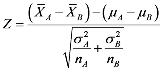 (2.1.1)
Required sample size in each treatment group for comparing two independent groups is calculated as following way [5,8-11]:
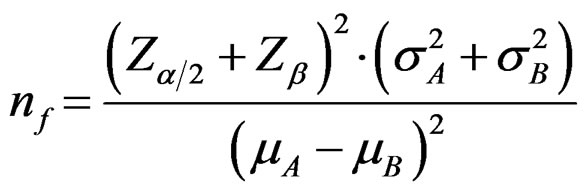 (2.1.2)
2.2. Group Sequential Designs
In group sequential designs, number of analysis (K) and required sample size (m) in each group for each analysis is determined initially while two treatments are comparing. Total number of analyses in a group sequential design is K, consisting of K – 1 interim analyses and a final analysis. The maximum subject number enroll to study is 2mK. The formula of Zk statistic to compare two means if A and B distributing normally with a known variance, and including 2m subjects is as follow [5,9]:
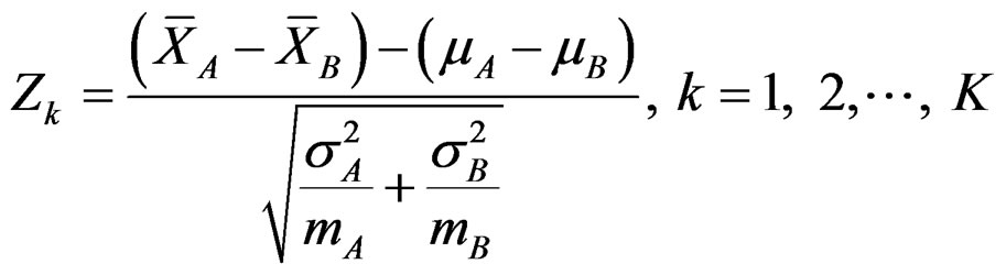 , (2.2.1)
Maximum sample sizes for each test types are differrent and calculated by multiplying nf in Equation (2.1.2) with a special factor R varying for each test type and each number of analysis.
In group sequential designs, since the number of statistical analyses is more than one, to protect total Type I error rate (α), Type I error rate (αk) for each analysis should be determined by allocating the total Type I error rate (α) to each analysis. And the ck critical values are determined according to these Type I error rates (αk) [1-3, 5,12]. Interim analyses are done after collecting data from each 2m subjects groups periodically and Zk test statistic is calculated for each analysis. When the value of Zk statistic calculated is equal to or larger than ck critical value the null hypothesis (H0) is rejected and the trial is terminated, referring as “positive result”. If the value of Zk statistic calculated is less than ck critical value, the trial continuing by adding a new 2m subjects group. If there is no positive result until final analysis and if still Zk < ck at the final analysis, than trial is terminated accepting the null hypothesis, referring as “negative result” [1,3, 5,9].
2.2.1. Pocock Test
The value of Z statistic after each interim analyses and final analysis is calculated with the formula given at Equation (2.2.1). The critical values of Pocock test that compared with the value of Z statistics are denoted as . The critical values
  varying based on total Type I error rate (α) and number of analyses (K), and remain constant for all interim analyses and final analysis [5,9].
The maximum sample size for Pocock test is calculated by multiplying nf in Equation (2.1.2) with
 values. The
  values varying based on total Type I error rate (α), Type II error rate (β) and number of analyses (K). Subject number for each treatment in each interim analysis is calculated as follow [5,9]:
 (2.2.2)
2.2.2. O’Brien & Fleming Test
The value of Z statistic after each interim analyses and final analysis is calculated in the same way with the formula given at Equation (2.2.1). The critical values of O’Brien & Fleming test that compared with the value of Z statistics are denoted as  for final analysis. For interim analyses, the critical values are obtained by multiplying
  with
with . The critical values
  varying based on total Type I error rate (α) and number of analyses (K), and are different for each interim analyses and final analysis [5,9]:
The maximum sample size for O’Brien & Fleming test is calculated by multiplying nf in Equation (2.1.2) with  values. The
  values varying based on total Type I error rate (α), Type II error rate (β) and number of analyses (K). Subject number for each treatment in each interim analysis is calculated as follow [5,9]:
 (2.2.3)
2.2.3. Wang & Tsiatis Test
There is a  parameter for Wang & Tsiatis test differently from other tests and certain values of this parameter makes Wang & Tsiatis test the same with Pocock and O’Brien & Fleming tests. Wang & Tsiatis test is same with Pocock test when
  and with O’Brien & Fleming test when
 . Values of
  between 0 - 0.5 gives critical values between Pocock and O’Brien & Fleming tests. Also, the value of Z statistic after each interim analyses and final analysis is calculated with the formula given at Equation (2.2.1). The critical values of Wang & Tsiatis test that compared with the value of Z statistics are denoted as
  for final analysis. For interim analyses, the critical values are obtained by multiplying
  with
with . The critical values
  varying based on total Type I error rate (α) and number of analyses (K), and are different for each interim analyses and final analysis [5, 9].
The maximum sample size for Wang & Tsiatis test is calculated in the same manner by multiplying nf in Equation (2.1.2) with  values. The
 values vary based on total Type I error rate (α), Type II error rate (β), number of analyses (K) and value of
 . Subject number for each treatment in each interim analysis is calculated as follow [5,9].
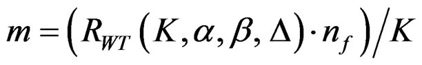 (2.2.4)
2.2.4. Haybittle-Peto Test
Calculation of Z statistic after each interim analyses and final analysis is the same with other tests, with the formula given at Equation (2.2.1). Haybittle-Peto test suggested that, in  analyses, namely in all interim analyses, H0 can be rejected only if
 . So, critical values of this test denoted as
  are constant (
 ) for all interim analyses. It is different only for final analysis The critical values
  for final analysis is varying based on total Type I error rate (α) and number of analyses (K) [5,9].
The maximum sample size for Haybittle-Peto test is calculated by multiplying nf in Equation (2.1.2) with  values. The
  values vary based on total Type I error rate (α), Type II error rate (β) and number of analyses (K). Subject number for each treatment in each interim analysis is calculated as follow [5,9].
 (2.2.5)
2.3. Models
In this study, four test types (Pocock, O’Brien & Fleming, Wang & Tsiatis and Haybittle-Peto tests) used to test difference between to treatment in group sequential designs were compared with fixed sample size design test and each other. In this sense, 10080 models were performed. In models, 2 different Type I errors (α), 2 different powers (1-β), 14 different number of analyses (K), 15 different effect sizes (d) and 12 different variances (σ2) selections were considered:


Sample size calculations for large effect sizes were too small and critical values according to analysis group numbers can be calculated by iteration [5,13], so 1080 of these 10080 models were used. In these models, 2 different Type I errors (α), 2 different powers (1-β), 5 different number of analyses (K), 6 different effect sizes (d) and 9 different variances (σ2) selections were considered:

Critical values to reject null hypothesis (H0) and maximum sample sizes required for all test types were determined for each combination. In each combination, these four test types were compared with each other and fixed sample size design test, and advantages and disadvantages of tests were examined in same conditions. Haybittle-Peto and Wang & Tsiatis tests can only be used for  Type I error rate [5,13]. So, these tests were only compared for
  combinations. In other combinations, only Pocock and O’Brien & Fleming test were compared with each other and fixed sample size design test. In addition, critical values of all test types decreasing from first interim analysis to final analysis. So, critical values for different number of analysis not included in tables can be calculated by iteration [5,13]. Results are summarized with tables.
3. Results
Critical values of each test types to reject null hypothesis (H0) at  level were shown at Tables 1-4. Also, sample size calculations for each test types to detect 3 different effect sizes with 6 several variances at 2 different 1 – β level and
  level were shown at Tables 5-10. Since Haybittle-Peto and Wang & Tsiatis tests can only be used at
  level, comparisons at
  level were done only for Pocock and O’Brien & Fleming tests. Advantages and disadvantage of these tests according to each other at
  level were same with the condition at
  level. So, results of
  level combinations were not shown. In addition, sample sizes calculated for larger effect sizes were very small as 3.9 and some of them not possible in practice. Thereby some of these sample sizes were similar and not comparable. So, sample sizes for
 ,
,  and
and  were not shown. Sample sizes calculated according to different variance selections increasing as variances increase and can be calculated by iteration. So, sample sizes for
 ,
,  , and
, and
 were not shown.
Critical value of fixed sample size design test to reject null hypothesis (H0) at  level is
 . The nearest critical value of group sequential tests at final analysis was obtained for Haybittle-Peto test and the furthest one was obtained for Pocock test. And it did not change according to the number of analysis (Tables 1-4).
When , Pocock test had the lowest critical values that might detect smaller effect sizes in first three interim analyses while O’Brien & Fleming test had the lowest critical values that might detect smaller effect sizes at 4th interim analysis and final analysis. This changing was observed at 7th interim analysis when
 , at 10th interim analysis when
  and at 13th interim analysis when
 . Wang & Tsiatis test was always placed between these two tests. It was closed to O’Brien & Fleming test for small
  values and started to close up to Pocock with increasing
  values. Critical values of Wang & Tsiatis test for early interim analyses were getting closer to Pocock test as the
  values increase, and they were decreasing for later interim analyses. Similarly, critical values of Wang & Tsiatis test were getting closer to O’Brien & Fleming test as the
  values decrease, and they were decreasing for later interim analyses in parallel with critical values of O’Brien & Fleming test. When
 , Pocock test had lower critical values that might detect smaller effect sizes than Wang & Tsiatis test for all
  values in first two or three interim analyses, while Wang & Tsiatis test had lower critical values that might detect smaller effect sizes in last two interim analyses and final analysis. This changing was observed at 5th - 7th interim analysis when
 , at 7th - 10th interim analysis when
  and at 8th - 11th interim analysis when
 . Number of analysis which this changing was observed, was varying according to value of
 . Haybittle-Peto test had a different way as having a constant critical value for all interim analysis. This critical value was placed between critical values of Pocock and O’Brien & Fleming tests for early interim analyses, and became higher from them after a few interim analysis. This changing was observed at 3rd interim analysis when
 , at 5th interim analysis when
 , at 8th interim analysis when
  and at 11th interim analysis when
 . Only for final analysis Haybittle-Peto test had a different critical value that the nearest one to fixed sample size design test (Tables 1-4).
All of the group sequential tests were required more sample size than the fixed sample size designs (Tables 5-10). This increase was depending on effect size. Difference between sample sizes for group sequential tests and fixed sample size design was minimal when the effect size was large. Even they were similar beginning from .
.

Table 1. Critical values for α = 0.05 and K = 5.
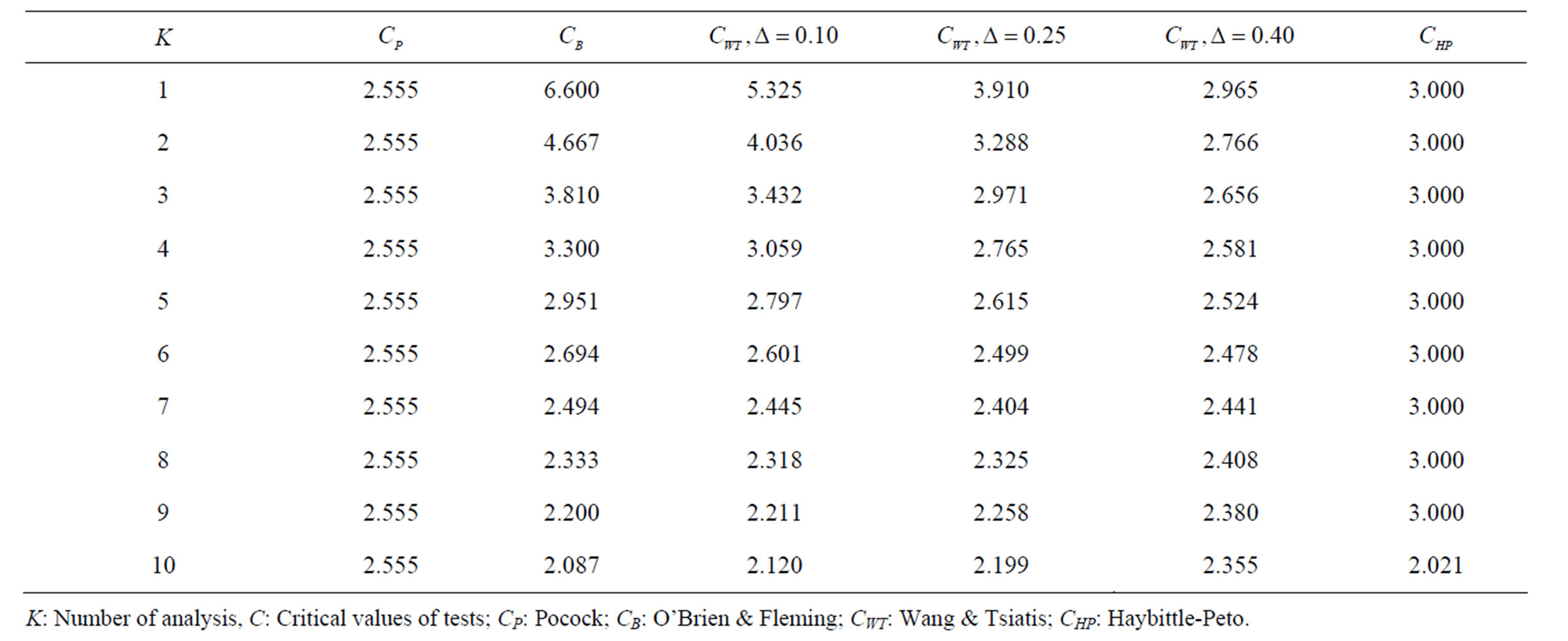
Table 2. Critical values for α = 0.05 and K = 10.
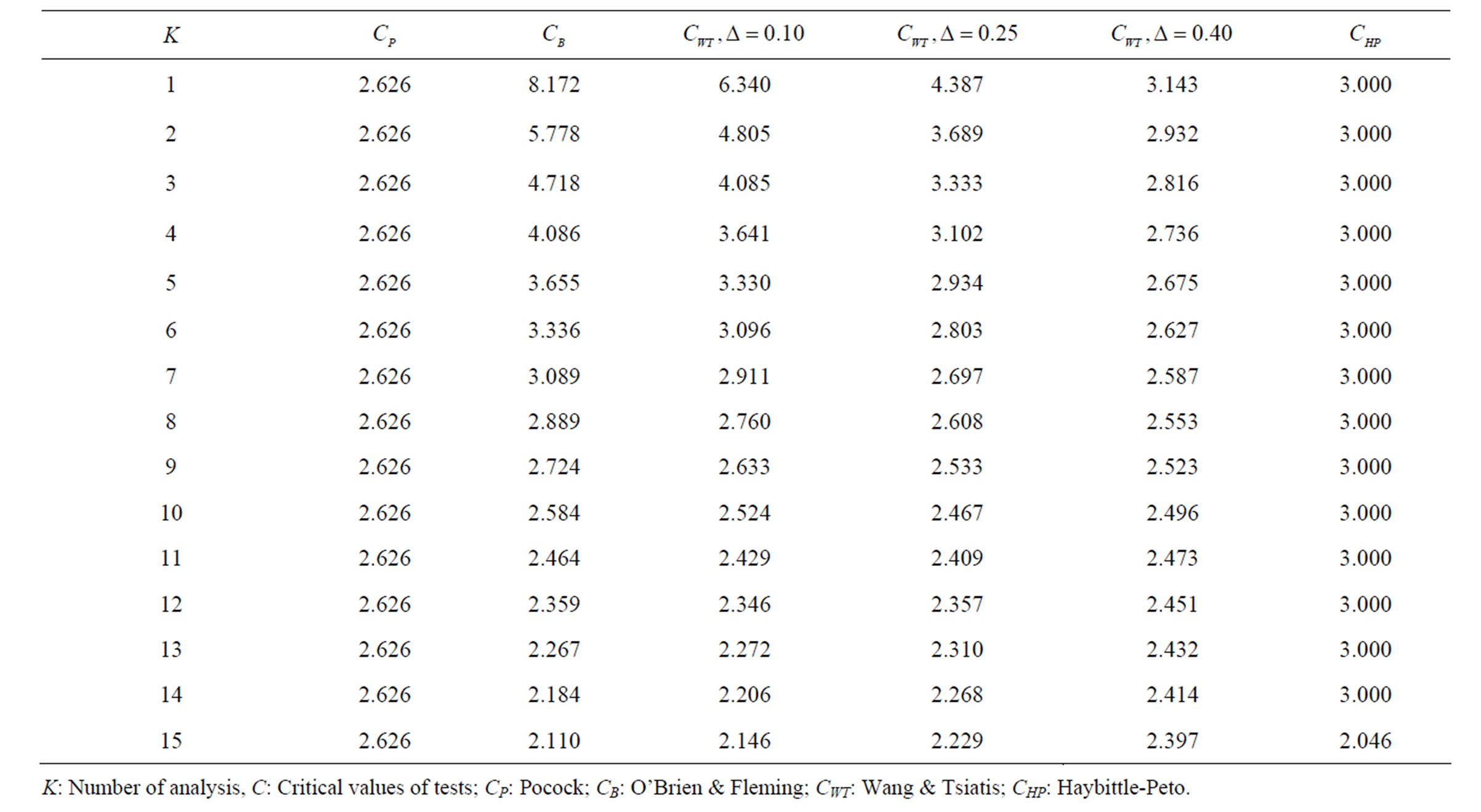
Table 3. Critical values for α = 0.05 and K = 15.
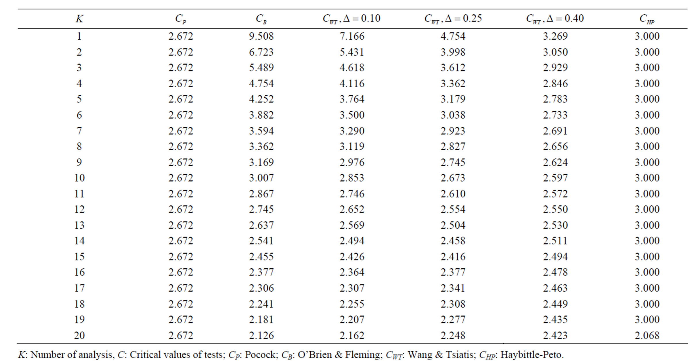
Table 4. Critical values for α = 0.05 and K = 20.
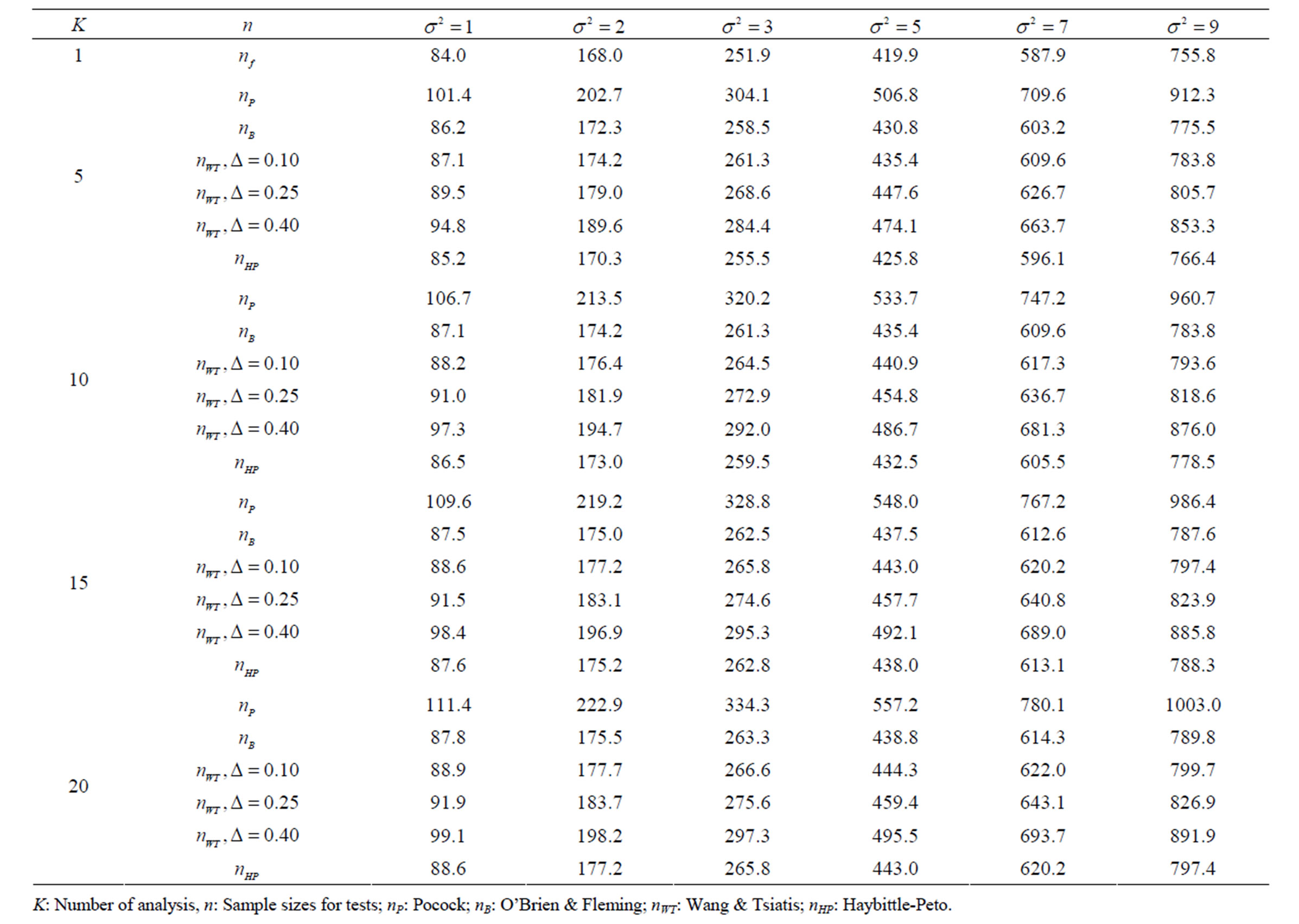
Table 5. Sample sizes for α = 0.05, (1 – β) = 0.90, and d = 0.5.
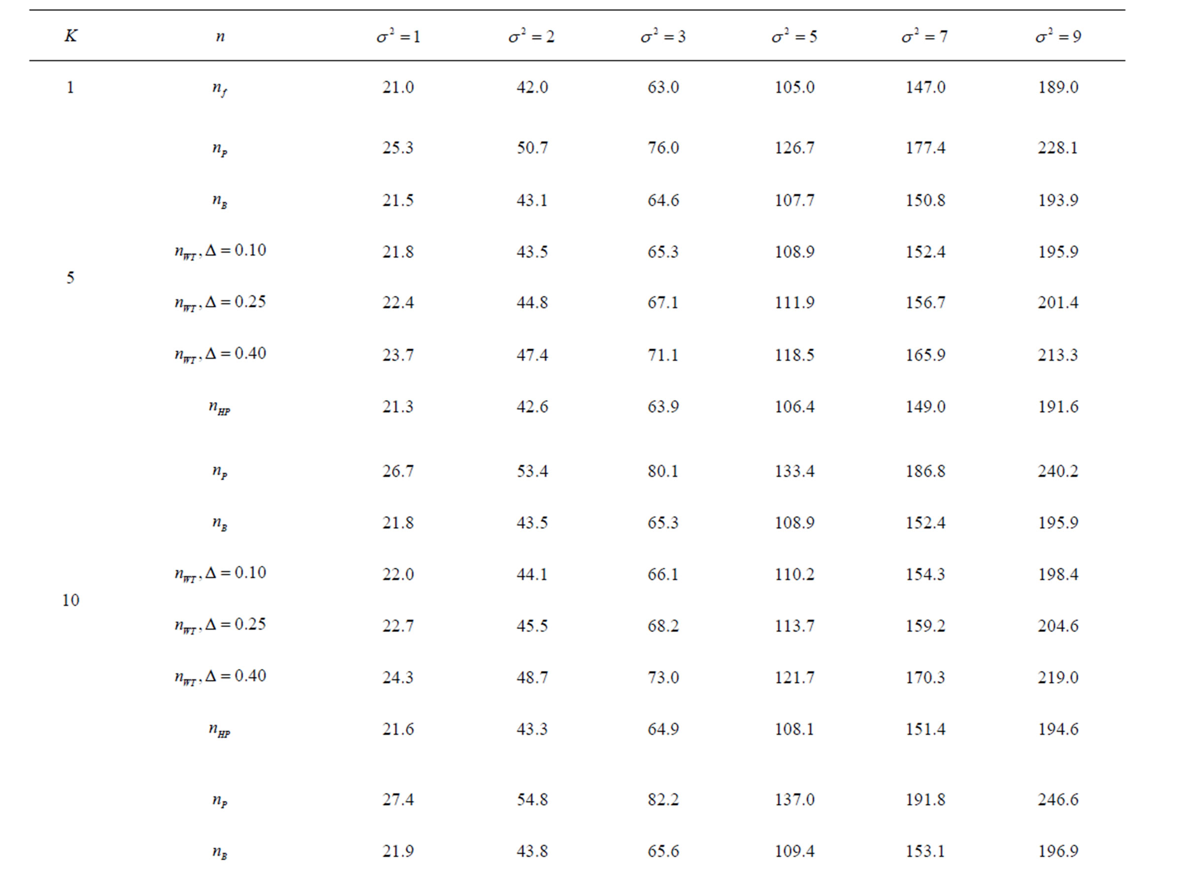
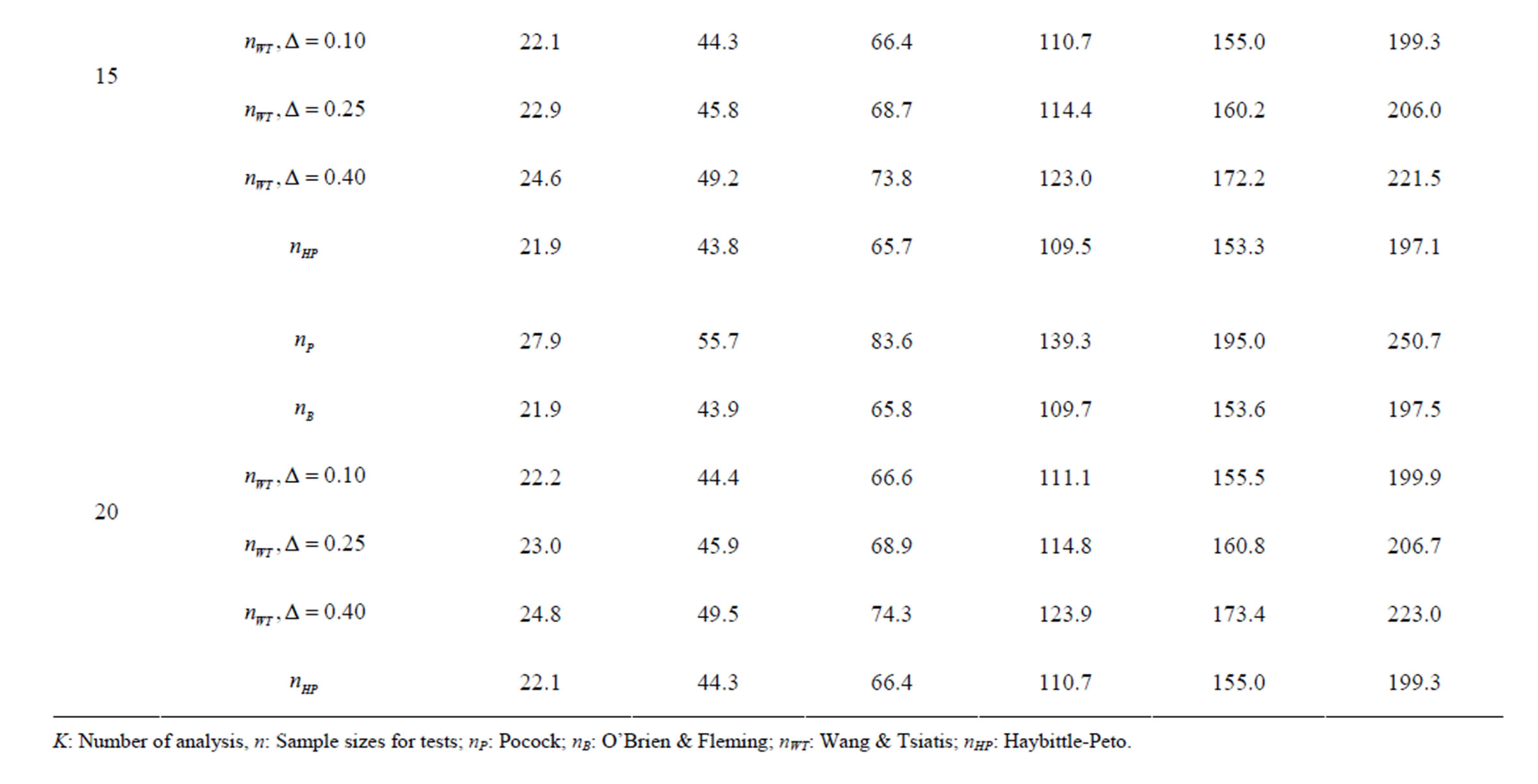
Table 6. Sample sizes for α = 0.05, (1 – β) = 0.90, and d = 1.0.
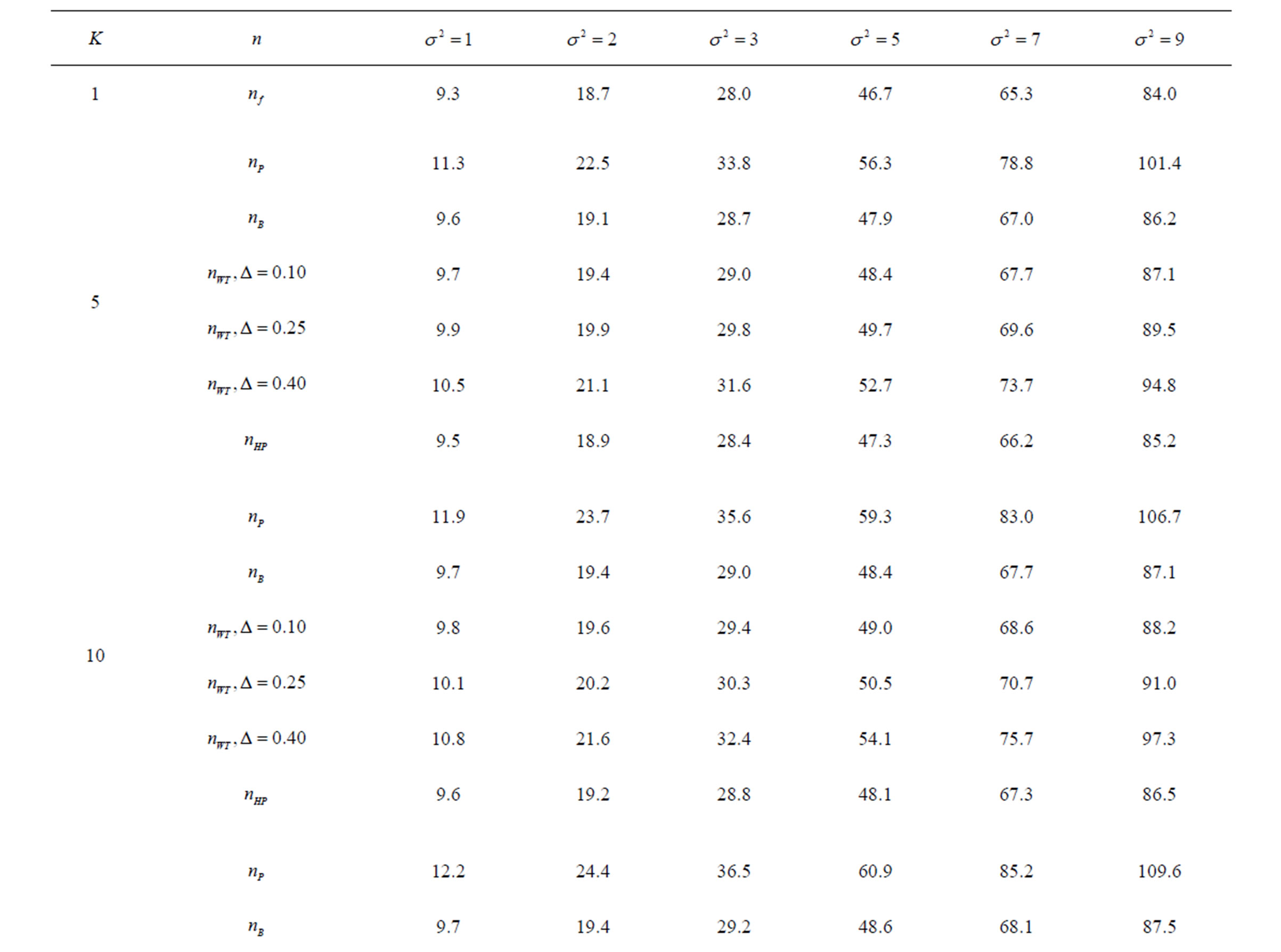
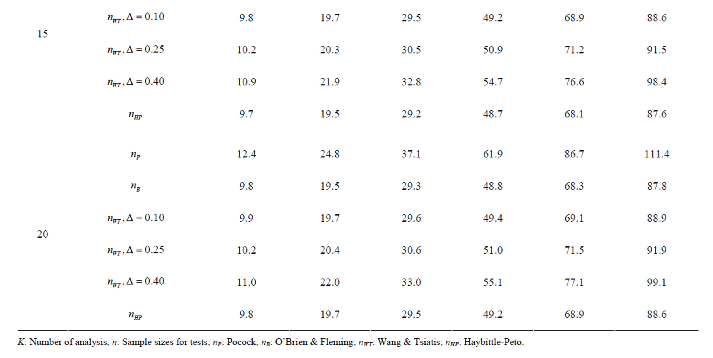
Table 7. Sample sizes for α = 0.05, (1 – β) = 0.90, and d = 1.5.
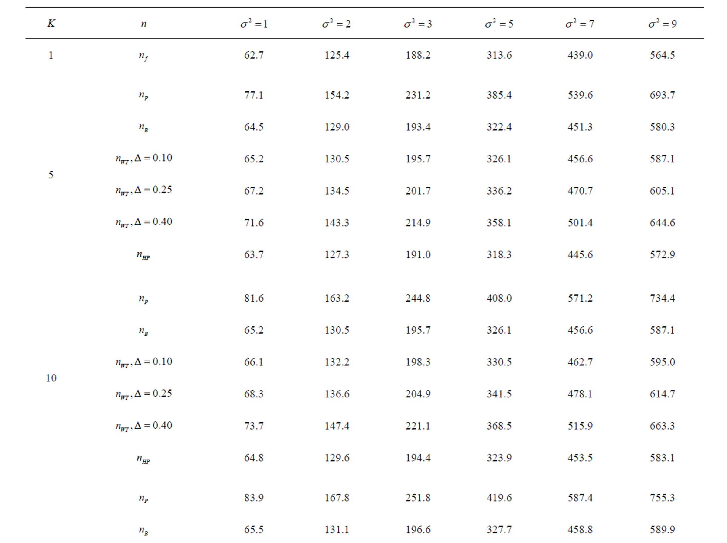
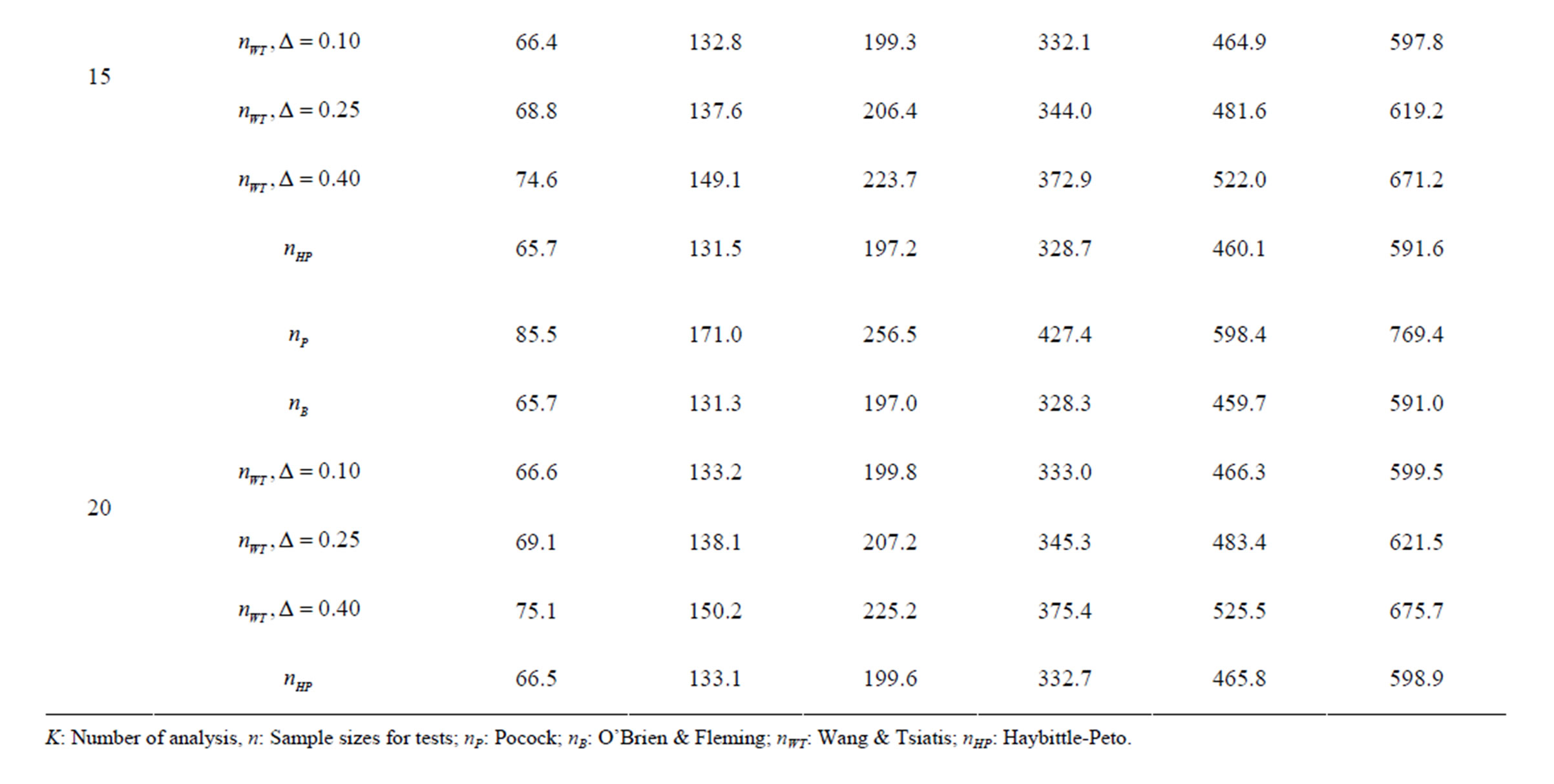
Table 8. Sample sizes for α = 0.05, (1 – β) = 0.80, and d = 0.5.
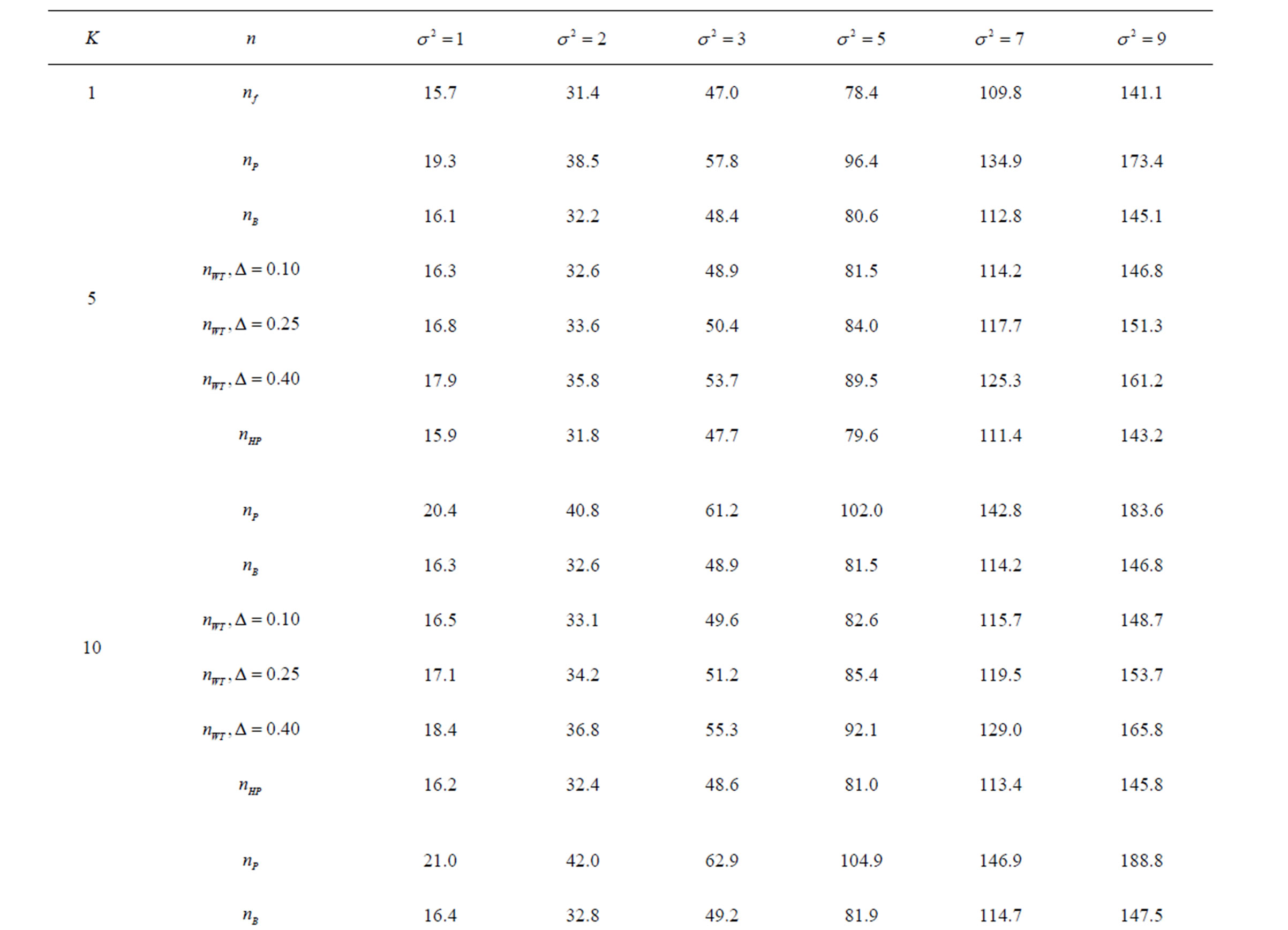
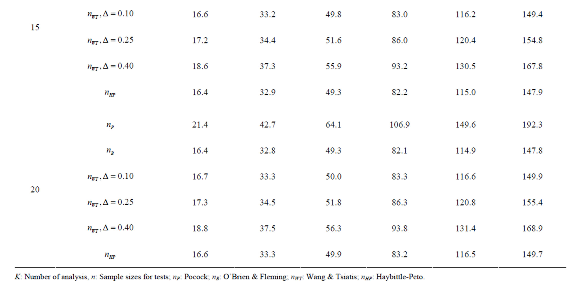
Table 9. Sample sizes for α = 0.05, (1 – β) = 0.80, and d = 1.0.
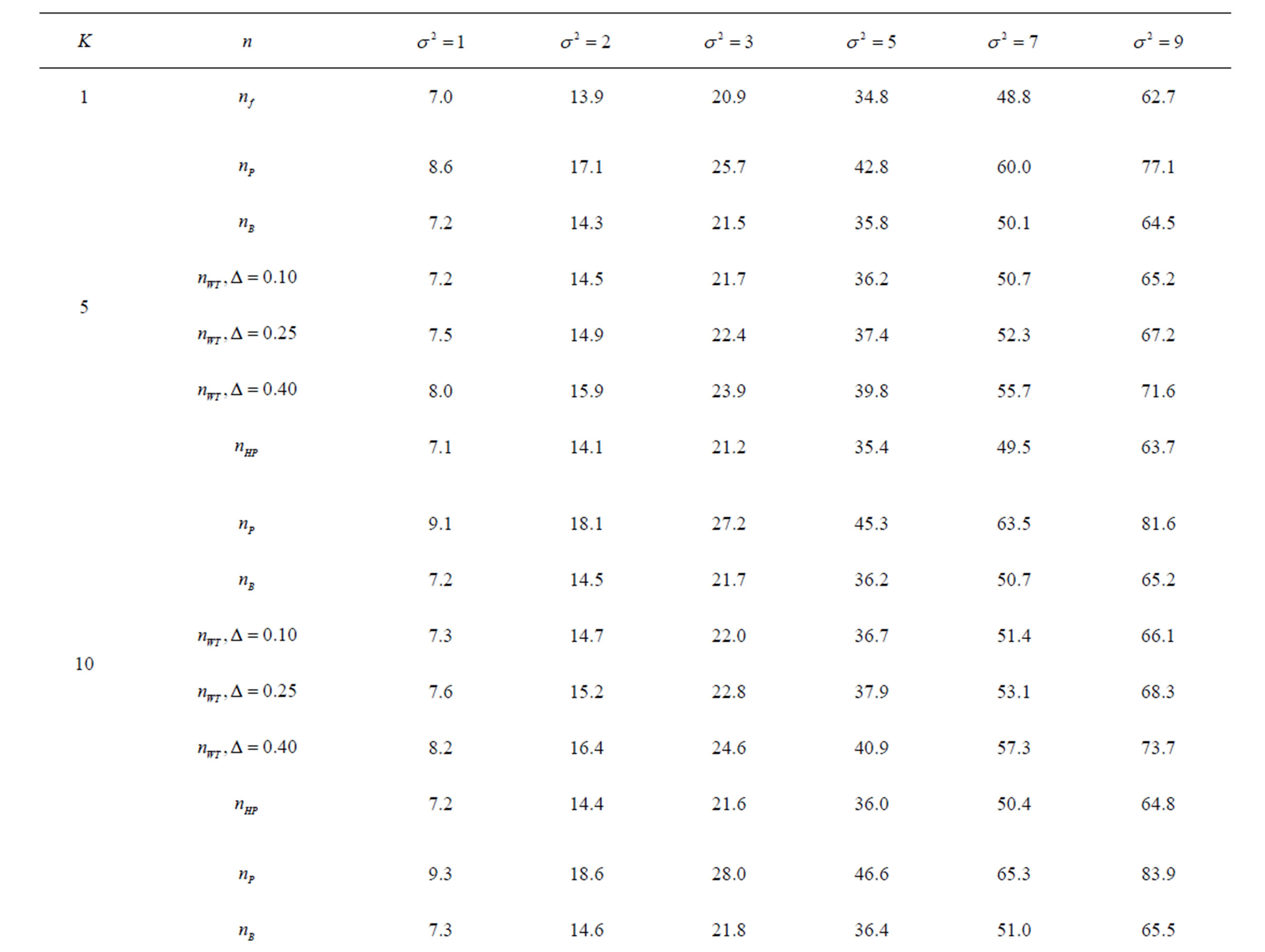
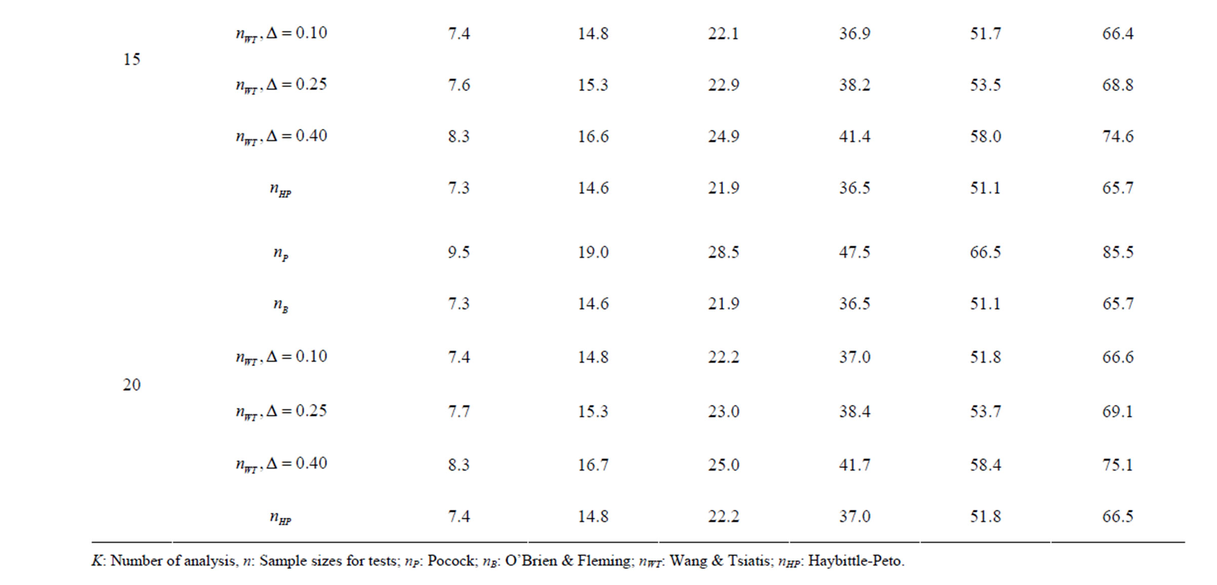
Table 10. Sample sizes for α = 0.05, (1 – β) = 0.80, and d = 1.5.
Pocock test required the largest sample size among the group sequential test types. O’Brien & Fleming and Haybittle-Peto tests had nearest sample sizes to fixed sample size design and order of these two tests changed with number of analyses. For example, when  Haybittle-Peto test had the smallest sample size while O’Brien & Fleming test required the smallest sample size when
 . But Pocock test had always the largest sample size for all combinations. Wang & Tsiatis test was always placed between these two tests as for critical values. It had the same sample size with Pocock test when
  and with O’Brien & Fleming test when
 . The sample size was close to O’Brien & Fleming test for small
  values and started close to Pocock test with increasing
  values. This condition was not varying according to number of interim analysis and other parameters related to calculation of sample size, as power, Type I error rate, effect size and variance. Sample sizes were almost similar for increasing effect sizes, and became same at
  and more effect sizes. It was mainly caused by the smallness of sample sizes such as 3.9. Because of the smallness of sample sizes, the differrences between sample sizes for each test can not be observed and they were seen similar. So, advantage and disadvantage of each test in term of sample size can be compared for low effect sizes.
4. Discussion
Results obtained about sample size in all combinations almost same. Haybittle-Peto and O’Brien & Fleming tests have been required much smaller sample sizes comparing to other test types. Pocock test has been required the largest sample size for all combinations. Wang & Tsiatis test has been always required sample size that placed between O’Brien & Fleming and Pocock tests.
The reason for requiring small sample size of O’Brien & Fleming test comparing to Pocock test, can be understood from the formula for calculating the Z statistic, Equality (2.2.1). It can be seen that, effect of effect size on expected value of test statistic  increases with number of analysis. So, the power of test achieves mainly later analyses [4,5].
Maximum sample size requiring in group sequential designs increases as the number of analyses increase. But, basic goal of group sequential designs is evaluating the advantage of early stopping through interim analysis [6,7, 13]. It takes into consideration that, maximum sample size is only required when there is no positive result in all interim analyses and the trial goes on to the final analyses.
Critical values of group sequential tests in interim analyses were ordered in a different manner, changing for each interim analysis. In addition, order of tests in term of critical values changing according to number of analysis (K). Pocock test had the lowest critical values for early interim analyses while O’Brien & Fleming test had the lowest critical values for latter analyses. Number of interim analysis in which this changing occurred varied according to number of analysis (K).
 values increase because of increase in
  values, and so the difference in critical values according to other tests in initial interim analyses increase as planned total number of analyses (K) increase.
  values start to decrease from first analysis to final analyses and therefore
  values start to decrease, so the critical values according to other tests are lower in latter analyses. Similarly, Wang & Tsiatis test shows same manner for critical values.
  values increase because of increase in
  values in initial interim analyses as planned total number of analyses (K) increase, and there is a big difference in terms of critical values according to other tests. It starts to decrease as the analyses goes on, and lower than other tests in latter analysis.
The number of analyses performed is important as the test type used. In some conditions, 1 or 2 interim analyses may be effective for decreasing sample size, and generally 4 or 5 interim analyses are sufficient. Accordingly, for a group sequential design using O’Brien Fleming test,  interim analyses have been the optimum. In addition, for a group sequential design using Pocock test,
  interim analysis seems unreasonable.
As a result, these four test types have several advantages and disadvantages. In a group sequential trial, decision of test type using to analysis the trial data, based on a few criteria: 1) whether early termination is important or not; 2) reducing sample size; 3) the issue of trial; 4) whether reaching the subject easy or not; 5) detecting minimal effect sizes. In the conditions that, reaching subjects is hard or studying smaller sample size because of high risk, the test which provides that detect smaller treatment differences at the first interim analyses can be preferred.
REFERENCES
- D. L. DeMets, “Sequential Designs in Clinical Trials,” Cardiac Electrophysiology Review, 1998, Vol. 2, No. 1, pp. 57-60. doi:10.1023/A:1009954810211
- S. C. Chow and J. P. Liu, “Design and Analysis of Clinical Trials: Concepts and Methodologies (Wiley Series in Probability and Statistics),” 2nd Edition, Wiley-Blackwell, Hoboken, 2004.
- P. C. O’Brien, “Data and Safety Monitoring,” In: P. Armitage and T. Colton, Eds., Encyclopedia of Biostatistics, Vol. 2, 2005, pp. 1362-1371.
- R. Aplenc, H. Zhao, T. R. Rebbeck and K. J. Propert, “Group Sequential Methods and Sample Size Savings in Biomarker-Disease Association Studies,” Genetics, Vol. 163, 2003, pp. 1215-1219.
- C. Jennison and B. W. Turnbull, “Group Sequential Methods with Applications to Clinical Trials,” Chapman & Hall/CRC, Boca Raton, 2000.
- M. Mazumdar and A. Liu, “Group Sequential Design for Comparative Diagnostic Accuracy Studies,” Statistics in Medicine, Vol. 22, No. 5, 2003, pp. 727-739. doi:10.1002/sim.1386
- M. Mazumdar, “Group Sequential Design for Comparative Diagnostic Accuracy Studies: Implications and Guidelines for Practitioners,” Medical Decision Making, Vol. 24, No. 5, 2004, pp. 525-533. doi:10.1177/0272989X04269240
- B. Tasdelen and E. A. Kanik, “The Formulae and Tables to Determine Sample Sizes for Classical Hypothesis Tests,” University of Mersin School of Medicine Medical Journal, Vol. 4, 2004, pp. 438-446.
- S. C. Chow, J. Shao and H. Wang, “Sample Size Calculations in Clinical Research,” Marcel Dekker, Inc., New York, 2003.
- J. M. Lachin, “Sample Size Determination,” In: P. Armitage and T. Colton, Eds., Encyclopedia of Biostatistics, Vol. 7, 2005, pp. 4693-4704.
- E. Lakatos, “Sample Size Determination for Clinical Trials,” In: P. Armitage and T. Colton, Eds., Encyclopedia of Biostatistics, Vol. 7, 2005, pp. 4704-4711.
- H. H. Muller and H. Schafer, “Adaptive Group Sequential Designs for Clinical Trials: Combining the Advantages of Adaptive and of Classical Group Sequential Approaches,” Biometrics, Vol. 57, No. 3, 2001, pp. 886-891. doi:10.1111/j.0006-341X.2001.00886.x
- T. G. Karrison, D. Huo and R. Chappell, “A Group Sequential, Response-Adaptive Design for Randomized Clinical Trials,” Controlled Clinical Trials, Vol. 24, No. 5, 2003, pp. 506-522. doi:10.1016/S0197-2456(03)00092-8