American Journal of Computational Mathematics
Vol. 3 No. 2 (2013) , Article ID: 33544 , 10 pages DOI:10.4236/ajcm.2013.32021
A Wavelet Multigrid Method Using Symmetric Biorthogonal Wavelets
Department of Mathematics, California State University, Fresno, USA
Email: doreendl@csufresno.edu
Copyright © 2013 Doreen De Leon. This is an open access article distributed under the Creative Commons Attribution License, which permits unrestricted use, distribution, and reproduction in any medium, provided the original work is properly cited.
Received March 24, 2013; revised April 25, 2013; accepted May 23, 2013
Keywords: Multigrid; Wavelets; Biorthogonal Wavelets
ABSTRACT
In [1], the author introduced a wavelet multigrid method that used the wavelet transform to define the coarse grid, interpolation, and restriction operators for the multigrid method. In this paper, we modify the method by using symmetric biorthogonal wavelet transforms to define the requisite operators. Numerical examples are presented to demonstrate the effectiveness of the modified wavelet multigrid method for diffusion problems with highly oscillatory coefficients, as well as for advection-diffusion equations in which the advection is moderately dominant.
1. Introduction
It is well known that the multigrid method is very useful in increasing the efficiency of iterative methods used to solve systems of algebraic equations approximating partial differential equations. However, when confronted by certain problems, for example diffusion problems with discontinuous or highly oscillatory coefficients, the standard multigrid procedure converges slowly, with a rate dependent on the initial mesh size, or may even break down.
In [2], the wavelet transform, which uses both highand low-pass filter operators, is used to derive a new approach for the two-level multigrid method, under the assumption that the matrix on the fine grid is symmetric. Some one-dimensional examples are also examined in that paper. In [1,3], the author extended the results of this approach to two dimensions and to multiple-level multigrid, dropping the assumption of a symmetric fine grid operator. This approach was considered for several reasons. First, in [4], the authors investigate similarities between multiresolution analyses and multigrid methods, which similarities motivate investigation into waveletbased multigrid methods. In addition, in [5], for example, it is shown that a wavelet coarse grid operator defined by a Schur complement provides a good approximation to the homogenized coarse grid operator, and, as stated in [1,3], homogenization has been used to improve convergence of multigrid methods for diffusion problems with periodic coefficients (e.g., [6-9]) because the homogenized operator provides a very good approximation of the important properties (e.g., eigenvalues and eigenfunctions) of the original fine grid operator. Also a wavelet coarse grid operator defined by a Schur complement has a natural connection to the interpolation and restriction operators. Furthermore, wavelets can be applied to problems with periodic as well as non-periodic coefficients. Finally, the application of wavelet operators to vectors and matrices maintains the properties of the original problem.
Recently, symmetric biorthogonal wavelets have received attention for use in image compression (see, e.g., [10,11]), based on the lifting scheme developed by Sweldens in [12]. In fact, symmetric biorthogonal wavelets are the basis for lossless compression in the JPEG 2000 standard (see, e.g., [13]). In addition, using biorthogonal wavelets to define multigrid methods has been explored in other papers. For example, in [14], the authors use biorthogonal wavelets adapted to a differential operator with constant coefficients, from which they develop a system of linear equations, and then use a biorthogonal two-grid method to solve. In [15], the authors consider solving ill-conditioned symmetric Toeplitz systems by using a two-grid method in which the interpolation and restriction operators are defined using the Cohen, Daubechies, and Feauveau (CDF) 9/7 symmetric biorthogonal wavelets. In [16], the authors use biorthogonal wavelets as preconditioners for an algebraic multigrid method which they use to solve various partial differential equations.
In this paper, the wavelet multigrid method introduced in [1] is modified by using symmetric biorthogonal wavelet transforms to define the requisite operators. The organization of this paper is as follows. In Section 2, some background on multigrid methods and wavelets is given. Section 3 discusses the wavelet multigrid method developed from the application of the biorthogonal wavelet transform to a general second order partial differential equation in two dimensions. In Section 4, numerical considerations are discussed. Section 5 presents some numerical results of applying the modified wavelet multigrid method using symmetric biorthogonal wavelets to two diffusion problems with highly oscillatory coefficients and to three advection-diffusion problems with moderately dominant advection. The rapid convergence, relatively independent of the initial mesh size, of the modified wavelet multigrid method using biorthogonal wavelets is demonstrated for these problems. For all numerical results in this paper, the V-cycle multigrid method is used with one iteration of the smoother for the coarsening and the correcting phases.
2. Background
2.1. Multigrid Methods
The problem we are concerned with solving is the system of linear equations
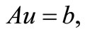 (1)
(1)
where  and
and  arise from discretization of a (partial) differential equation on some grid
 , where
  is the step size.
We briefly describe the V-cycle method used in this paper. Given some interpolation operator,  where the superscript refers to the fine grid and the subscript refers to the coarse grid, and a restriction operator,
  we can define a multigrid method recursively. For the two-level V-cycle method, we do the following.
Step 1: Relax a few (usually one or two) steps on the fine grid  to get an initial guess
 .
.
Step 2: Compute the residual 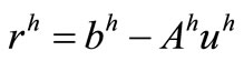 and restrict the residual to the coarse grid
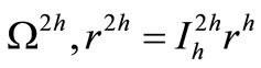 .
.
Step 3: Solve the error equation  on the coarse grid.
Step 4: Set 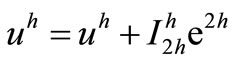 and again relax a few (usually one or two) steps on the fine grid.
Based on this two-level method, the V-cycle multigrid scheme is defined recursively. Some good references for multigrid methods are [17-19].
One type of multigrid scheme is algebraic multigrid, which only uses the structure of the matrix in the problem to determine the coarsening process (choice of coarse grid and definition of interpolation/restriction operators). This process is performed in order to ensure that the range of interpolation approximates the errors not sufficiently reduced via relaxation. For a more detailed description of algebraic multigrid methods, see, e.g., [19- 22]. Note that in [21] the relationship between algebraic multigrid and Schur complements is discussed. Algebraic multigrid methods are of particular interest, in that they are the nearest methods to the approach used for the wavelet multigrid method.
It is expected that the multigrid method should converge at a rate independent of the fine mesh size. However, for certain problems, including elliptic problems with highly oscillatory coefficients, such convergence does not occur for the standard multigrid method. One difficulty is that the small eigenvalues of A are not necessarily associated with smooth eigenfunctions, a key assumption for the standard multigrid method. For such problems, it is not as simple to approximate the smooth eigenfunctions on the coarse grids. New methods for restriction and interpolation, or for treating the entire problem, must be found. One such approach is the wavelet multigrid method discussed in [1,3] and the modified wavelet multigrid method discussed in this paper.
2.2. Wavelets and Biorthogonal Wavelets
For background, a brief description of wavelets, and then of biorthogonal wavelets, follows. For more details, the reader is referred to [10,23-25].
2.2.1. Wavelets
Wavelets basically separate data (or functions or operators) into different frequency components and analyze them by scaling. The wavelets can be chosen to form a complete orthonormal basis of . Due to the scaling of the wavelet functions, they have timeor spacewidths that are related to their frequency: at high frequencies, they are narrow, and at low frequencies, they are broader. Therefore, they provide good localization of functions in both the frequency domain and physical space, and representation by wavelets seems natural to apply to the analysis of fine and coarse scales.
A multiresolution analysis (MRA) consists of a sequence of closed subspaces  of
of , the scaling spaces, that satisfy certain conditions. For every
 is defined as the orthogonal complement of
  in
in  The
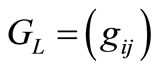
The  are called the wavelet spaces. Define
  and
and  to be the operators that transform the basis of the space
  to the bases of the spaces
  and
and , respectively. The properties of
  and
and  (assuming
  and
and  are real-valued) are
(i)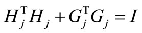 .
.
(ii) .
.
(iii) .
.
 and
and  can be thought of in terms of filter theory, with
  being a low-pass filter (i.e., allowing only low frequency values to pass) and
  being a high-pass filter (i.e., allowing only high frequency values to pass). The wavelet transform,
  , is defined by
Note that  is orthogonal due to the properties of
  and
and .
.
In the discrete context, the wavelet operators are computationally efficient. With respect to the Haar multiresolution analysis, application of the low-frequency operator  to a vector in
  involves only
  operations. The same holds for the high-frequency operator
 . So, the application of the wavelet transform requires only
  operations. In general, application of the wavelet transform requires
  operations, assuming a finite number of coefficients for the lowand high-frequency operators.
In two dimensions, the tensor product of one-dimensional multiresolution analyses is used. So  is defined by
 . These spaces
  then form an MRA in
 . For each
 ,
,  is defined as the orthogonal complement of
  in
in  So,
So,
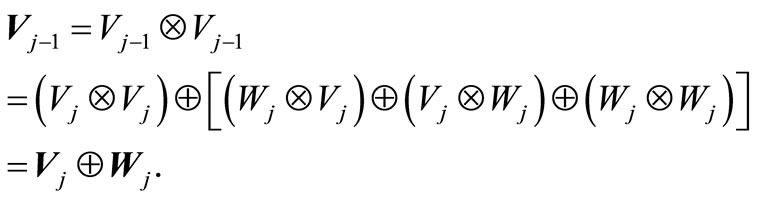 (2)
(2)
Then, analogous to the one dimensional case, define the operators  and
and  so that
and
 and
and  have the same properties as their onedimensional analogues. As in the one-dimensional case, the wavelet transform,
 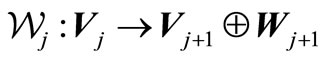 , is defined by

Again, due to the properties of  and
and ,
,  is orthogonal.
2.2.2. Biorthogonal Wavelets
A biorthogonal multiresolution analysis consists of two dual multiresolution analyses. In other words, there are two dual sequences of closed subspaces of ,
,
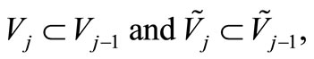
both of which satisfy the conditions of a multiresolution analysis. For every ,
,  can be written as the direct sum of
  and
and , and
, and  can be written as the direct sum of
  and
and .
.  and
and  are defined so that their biorthogonal basis functions, the wavelets
  and
and , respectively, satisfy certain conditions including forming a Riesz basis of
 . For symmetric biorthogonal multiresolution analyses, these wavelet bases (and the bases for the scaling spaces) are symmetric. Define
  and
and  to be the operators that transform the basis of the space
  to the bases of the spaces
  and
and , respectively; and define
  and
and  to be the operators that transform the basis of the space
  to the bases of the spaces
  and
and , respectively. The properties of
 ,
,  ,
,  and
and  are as follows:
(i)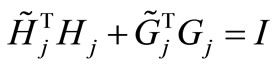 .
.
(ii)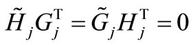 .
.
(iii)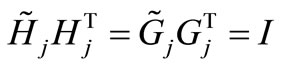 .
.
The wavelet transform, 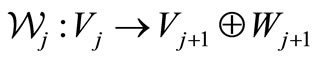 and the dual transform
  are defined by

where we use  to denote the direct sum for ease of notation. Note that
  is orthogonal to
  due to the properties of
 ,
,  ,
,  and
and . Also, note that in terms of filter theory,
  and
and  are low-pass filters, and
  and
and  are high-pass filters.
The discrete biorthogonal wavelet transforms are also computationally efficient, and application of these operators requires  operations, assuming a finite number of coefficients for the lowand high-frequency operators.
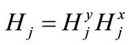
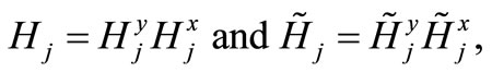
In two dimensions, we use the tensor product in a similar way as for the standard multiresolution analysis. So,  is defined by
  and
and  is defined by
 . These spaces
  and
and  then form dual MRAs in
 .
.  and
and  are defined so that their basis functions are the tensor products of the one-dimensional wavelets and scaling functions. For each
 ,
,  can be written as the direct sum of
  and
and , and
, and  can be written as the direct sum of
  and
and . So, we have
 (3)
(3)
and similarly for , where we again use
  to denote the direct sum for ease of notation.
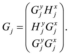
Then, analogous to the one-dimensional case, define the operators ,
,  ,
,  and
and  so that:
and
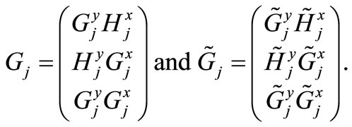
 have the same properties as their one-dimensional analogues. As in the one-dimensional case, the wavelet transform and the dual transform
  and
and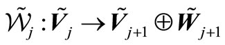 , are defined by

Again, due to the properties of ,
,  ,
,  and
and ,
,  is orthogonal to
 .
.
3. The Modified Wavelet Multigrid Method Using Biorthogonal Wavelets
The two-dimensional wavelet multigrid method was introduced in [3] and [1]. Both of these works assumed orthogonal wavelet operators. Here, we describe the modified wavelet multigrid method using biorthogonal wavelet transforms. For the work in this paper, the biorthogonal wavelet transform is formed using symmetric biorthogonal wavelets.
Given the problem
 (4)
(4)
where  represents the operator obtained by discretizing a two-dimensional partial differential equation on the fine grid, apply the wavelet transform
  to both sides of the equation and use the orthogonality of
  with
with  to obtain
 (5)
(5)
where  and
and
The main idea for the remainder of the method follows in a similar manner as the wavelet multigrid method using orthogonal wavelet transforms. First, 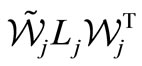 is computed, and the resulting matrix, denoted by
 , is partitioned to obtain
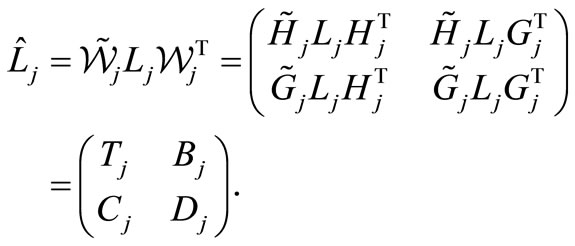 (6)
(6)
Then, the block UDL decomposition of , where U is block upper triangular with unit diagonal, D is block diagonal, and L is block lower triangular with unit diagonal, is computed and is used to find
  as follows. The block UDL decomposition of
  is determined to be
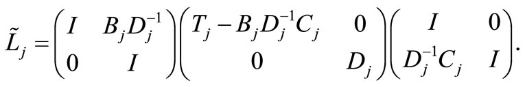 (7)
(7)
The inverse of this factorization of  is then computed, which after multiplication of the factors gives
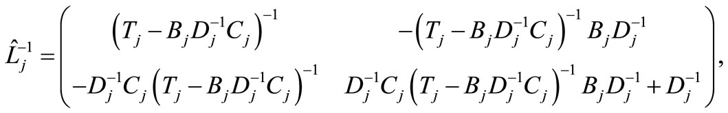
where we observe that  is the Schur complement of
  in
in . Define
Solving for  gives
gives

Since . So,
. So,
 (8)
(8)
Motivated by the work in [1], we denote
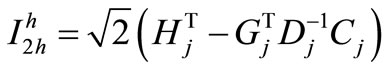 (9)
(9)
and
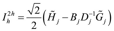 (10)
(10)
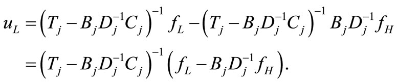
as the interpolation and restriction operators, respectively. Plugging the interpolation and restriction operators defined in (9) and (10) into (8) gives,
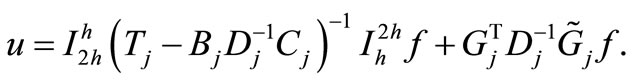 (11)
(11)
In multigrid, the error correction on the coarse grid is sought, i.e., the equation being solved is (11) with u replaced by the error, e, and f replaced by the residual, r:
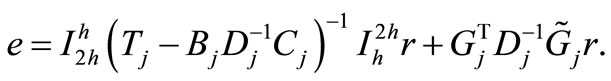
Assuming that 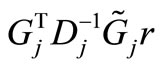 is small, i.e., r is almost in
  the error can be approximated by

resulting in
The above assumption is good for most of the classical iterative methods, like Jacobi and Gauss-Seidel. Therefore, the coarse grid operator is defined by
 (12)
(12)
which we again note is the Schur complement of  in
in 
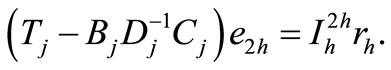
Note: This coarse grid operator is the same as the operator obtained by solving for :
:
The above procedure may be repeatedly applied until the desired coarseness is reached. Notice that this method is applicable to problems which are not symmetric. However, regardless of the discretization scheme used, the operator matrix must be a square matrix whose row size is a multiple of four.
4. Numerical Considerations
The main numerical issue is fill-in in the matrices as the multigrid method involves increasing levels in the Vcycle. Thresholding is used to reduce fill-in in the computation of . Furthermore, although
  is not dense, its inverse is dense due to fillin. However, a significant amount of decay is observed, indicating that it is possible to increase the efficiency of the method in this area.
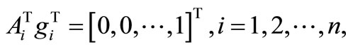
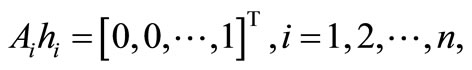
One step towards achieving this goal is to compute an approximate inverse using a factorized sparse approximate inverse. In this work, we use the approach suggested by Salkuyeh in [26]. Salkuyeh’s approach is based on Kolotilina and Yeremin’s factorized sparse approximate inverse algorithm, FSAI [27,28]. The goal is to determine a factorization of the form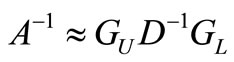 , where
  is upper triangular,
  is lower triangular, and D is diagonal. This approximation is determined by computing sparse approximate solutions to the systems of equations
 (13)
(13)
 (14)
(14)
where  denotes the ith principal submatrix of
 ,
,  , and
, and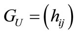 . In Salkuyeh’s paper, these systems are solved using a self-preconditioned minimum residual (MR) algorithm with dropping in the search direction (similar to that proposed by Chow and Saad in [29]), starting with an initial sparse guess for the solution and iterating while the solution has fewer than the specified number of nonzeros, denoted by the value lfil. In our work, lfil iterations of the MR algorithm are performed in order to avoid potential infinite loops. Then, structural requirements are enforced; namely, the inverse is required to have the same structure as the matrix
 . In addition, thresholding is used to further reduce the fill-in in the inverse.
4.1. Cost of Computing the Approximate Inverse
The bulk of the cost of the self-preconditioned MR algorithm with dropping in the search direction can be measured in terms of the sparse matrix-sparse vector products and the sparse vector-sparse vector products. One sparse matrix-sparse vector product is required to compute the initial residual, and each iteration of the algorithm requires one sparse matrix-sparse vector product and two sparse vector-sparse vector products.
The MR algorithm is used to compute sparse approximate solutions to the system in (13)-(14). For each i, these systems have coefficient matrices that are , where i ranges from 1 to
 , with
  the size of the matrix whose inverse is being computed. Thus, the MR algorithm is run
  times.
The final major contributions to the cost of the approximate inverse are the computation of (1) , which requires
  scalar inverses, and (2)
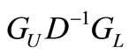 , which requires
  scalar products, where
  is the number of nonzero elements in
 , followed by one sparse matrix-sparse matrix product.
4.2. Computational Complexity of the Approximate Inverse
The following briefly examines the actual computational complexity of the approximate inverse for the wavelet multigrid method. The value of lfil used to construct the approximate inverse of  depends on the type of problem, the type of wavelet used, the fine grid size, and the level in the multigrid method. For all problems and wavelets, post-processing is done to ensure that
  has the same structure as
 , and thresholding is used on all matrices (except for
  for diffusion problems using Haar wavelets). Note that this is an improvement on the work in [1].
Thresholding values for the two diffusion examples in Section 5.1 are given in Tables 1 and 2. Note that the thresholding values for  and
and  for the 9/7 symmetric biorthogonal wavelets depend on the fine grid size and the level of the multigrid method. Similarly, the thresholding values for
  for Daubechies 4 wavelets depend on the fine grid size and the level of the multigrid method.
In terms of the lfil chosen for FSAI, for the diffusion problem with oscillations in the x-direction, for the modified wavelet multigrid method using 9/7 symmetric biorthogonal wavelets lfil ranges from 3 to 6, and using the 10/6 symmetric biorthogonal wavelets lfil ranges from 4 to 10. For that same problem, for the wavelet multigrid method using Haar wavelets lfil ranges from 9 to 11, and using Daubechies 4 wavelets lfil ranges from 3 to 10. For the diffusion problem with oscillation along diagonals, for the 9/7 symmetric biorthogonal wavelets lfil ranges from 1 to 6, and for the 10/6 symmetric biorthogonal wavelets lfil ranges from 1 to 9. For that same problem, using Haar wavelets lfil ranges from 4 to 11, and using Daubechies 4 wavelets lfil ranges from 3 to 10.
Thresholding values for the three advection-diffusion examples in Section 5.2 are given in Tables 3-5. Note that the thresholding values for  (and
(and  in the case of parabolic flow (9/7) and recirculant flow (10/6)) for the 9/7 and 10/6 symmetric biorthogonal wavelets depend on the fine grid size and the level of the multigrid method. Similarly, the thresholding values for
  (and
(and  in the case of recirculant flow) for Daubechies 4 wavelets depend on the fine grid size and the level of the multigrid method.
For the advection-diffusion problems with moderately dominant advection, for parabolic flow, for the modified wavelet multigrid method using 9/7 symmetric biorthogonal wavelets lfil ranges from 2 to 6, depending on the fine grid size and on the level of the multigrid, and using 10/6 symmetric biorthogonal wavelets, lfil ranges from 2 to 7. Using the wavelet multigrid method with Haar wavelets, lfil ranges from 2 to 12 and using it with Daubechies 4 wavelets, lfil ranges from 3 to 6. For recirculant flow, lfil ranges from 2 to 5 for 9/7 symmetric biorthogonal wavelets and from 2 to 4 for 10/6 symmetric biorthogonal wavelets, again depending on the fine grid size and on the level. For Haar wavelets, lfil ranges from 3 to 8, and for Daubechies 4 wavelets, it ranges from 2 to 10. For the problem with skewed vorticity, lfil ranges from 4 to 7 for 9/7 symmetric biorthogonal wavelets and from 2 to 6 for 10/6 symmetric biorthogonal wavelets. Using Haar wavelets, lfil ranges from 2 to 10, and using Daubechies 4 wavelets, it ranges from 4 to 9.
4.3. Storage and Other Computational Issues
The bulk of the remaining computational work occurs in the construction of the intergrid transfer and coarse grid operators. The construction of the intergrid transfer and coarse grid operators each requires two sparse matrixsparse matrix products and one sparse matrix-sparse matrix difference.
The storage requirements of the coarse grid and intergrid transfer operators are minimized by using sparse matrix storage techniques, resulting in storage requirements of the order of the number of nonzero elements in each matrix.

Table 1. Thresholding values for horizontal diffusion example in Section 5.1.

Table 2. Thresholding values for diagonal diffusion example in Section 5.1.

Table 3. Thresholding values for parabolic advection-diffusion example in Section 5.2.
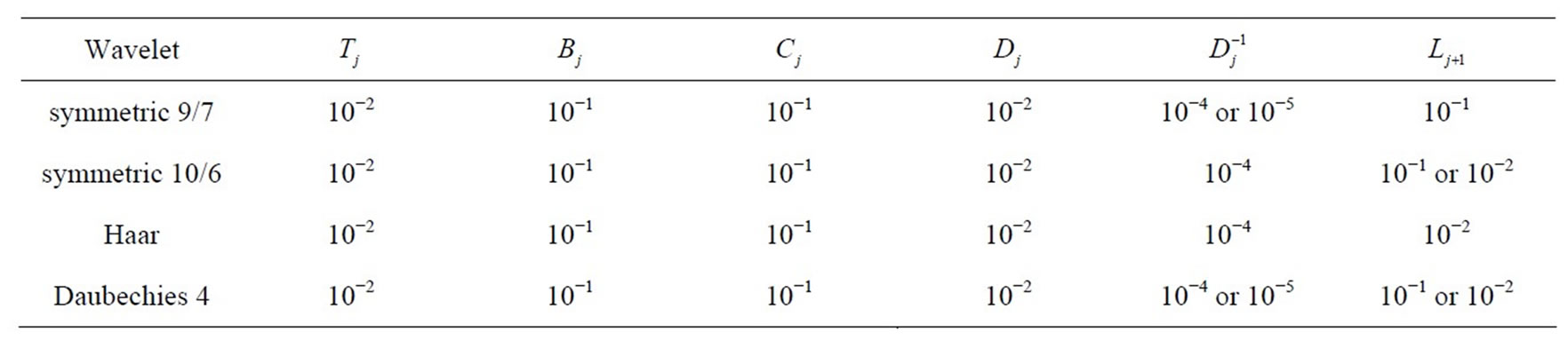
Table 4. Thresholding values for advection-diffusion example with recirculant flow in Section 5.2.
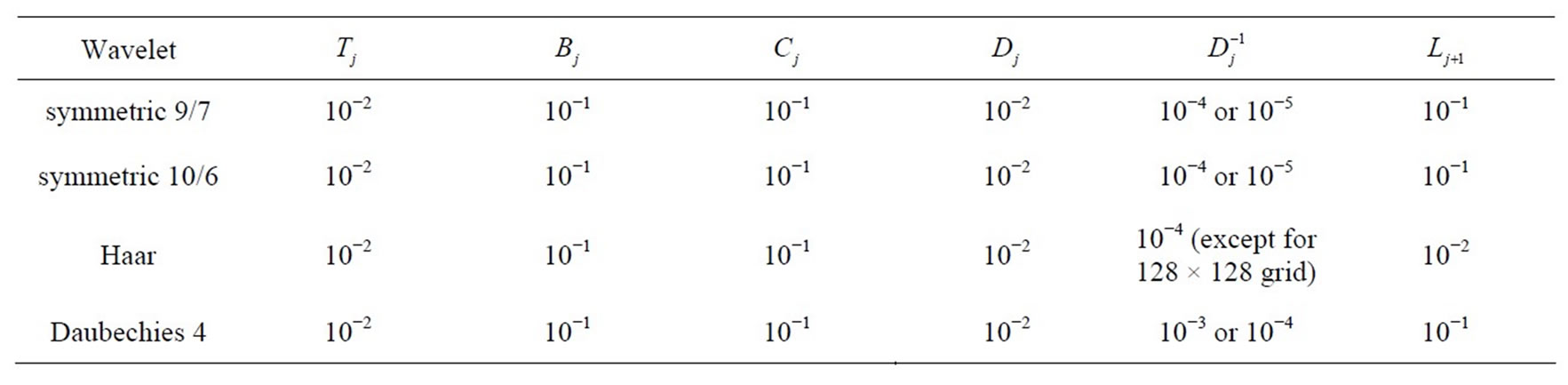
Table 5. Thresholding values for advection-diffusion example with skewed recirculant flow in Section 5.2.
5. Numerical Applications
This section describes the numerical results of applying the modified wavelet multigrid method using symmetric biorthogonal wavelets to two diffusion problems with highly oscillatory coefficients and to three advectiondiffusion problems with moderately dominant advection. We compare the convergence of the modified wavelet multigrid method using both 9/7 and 10/6 symmetric biorthogonal wavelets with the wavelet multigrid method using both Haar wavelets and Daubechies 4 wavelets. For all problems, numerical results are analyzed using, for the fine grid in the interior, a 32 × 32 grid, leading to a 1024 × 1024 matrix; a 64 × 64 grid, leading to a 4096 × 4096 matrix; and a 128 × 128 grid, leading to a 16384 × 16384 matrix. In all problems, the stopping criterion for all multigrid methods is , where
  is the residual obtained from the kth iteration of the method.
5.1. Diffusion Problems
First, we look at the diffusion problem
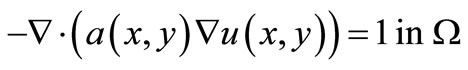 (15)
(15)

where  is the unit square centered at
  and
and  We will examine two cases where
  is a highly oscillatory function:
 giving oscillation in the x-direction, and
 , giving oscillation along diagonals. Results are examined using both 9/7 and 10/6 symmetric biorthogonal wavelets. The standard Gauss-Seidel iterative method is used as the smoother.
Tables 6 and 7 compare the average convergence factor per cycle of the modified wavelet multigrid method using symmetric biorthogonal wavelets with that of the wavelet multigrid method. These tables demonstrate results using a fixed coarsest grid size of 8 × 8 for each fine mesh size.
For the diffusion problem with oscillation in x, as well as the diffusion problem with oscillation along diagonals, the convergence of the modified wavelet multigrid method using symmetric biorthogonal wavelets is relatively independent of the fine grid size, as it is for the wavelet multigrid method using orthogonal wavelets. Convergence results for the method using both the 9/7 symmetric biorthogonal wavelets and the 10/6 symmetric biorthogonal wavelets are comparable to the results using the orthogonal wavelets for both problems.
5.2. The Advection-Diffusion Problem
Here, we are investigating the problem
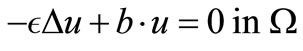 (16)
(16)

where  is the unit square centered at
  and
and . In this problem, difficulties with multigrid methods are encountered due to the fact that some of the components of the solution oscillate along characteristics [30,31]. We apply the wavelet multigrid method to these problems to overcome this difficulty, since application of the wavelet operator preserves the characteristics of the original problem.
To discretize, we use the standard five-point centered discretization for the diffusion term and a first order upwind scheme for the advection part of the equation. Although using first order upwind introduces artificial diffusion into the solution of the order of the mesh size squared, it provides a convenient test of the effectiveness of the modified wavelet multigrid method. Symmetric Gauss-Seidel is used as the smoother in order to ensure that sweeps are performed in the direction of the characteristics over the entire flow field. Results shown use 
First, we have a comparison of the methods for (16), where  and
and  is defined by
 (17)
(17)
Note that the discontinuous boundary condition will give rise to a boundary layer near the left-hand boundary. Also, the characteristics are parabolic, resulting in flow entering and exiting through the left-hand boundary. For both the modified wavelet multigrid method with symmetric biorthogonal wavelets and the wavelet multigrid method, convergence appears to be relatively independent of the fine mesh size, as can be seen in Table 8, which compares the average convergence factor per cycle using a coarsest grid size of 8 × 8.
In a second example,
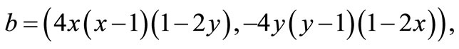
giving recirculant flow (i.e., closed characteristics), and  is defined in (17). The modified wavelet multigrid method using symmetric biorthogonal wavelets and the wavelet multigrid method both have a convergence rate that is relatively independent of the fine grid size. For this problem, the modified wavelet multigrid method
Table 6. Average convergence factor per cycle for diffusion problem with oscillation in x.

Table 7. Average convergence factor per cycle for diffusion problem with oscillation along diagonals.

Table 8. Average convergence factor per cycle for the advection-diffusion problem with parabolic characteristics and discontinuous boundary conditions.

Table 9. Average convergence factor per cycle for the advection-diffusion problem with recirculant flow and discontinuous boundary conditions.

Table 10. Average convergence factor per cycle for the advection-diffusion problem with skewed recirculant flow and discontinuous boundary conditions.
using 10/6 symmetric biorthogonal wavelets outperforms the wavelet multigrid method using both Haar wavelets and Daubechies 4 wavelets. The results are shown in Table 9, which compares the average convergence factor per cycle using a coarsest grid size of 8 × 8.
The final example uses the boundary conditions given by (17), but the advection component has both closed characteristics and a skewed flow, so that it does not line up with the grid. Here,

where
Both the modified wavelet multigrid method using symmetric biorthogonal wavelets and the wavelet multigrid method converge rapidly, with a convergence rate that is relatively independent of the fine grid size, as shown in Table 10, which displays the average convergence factor per cycle for the modified wavelet multigrid method using both 9/7 and 10/6 symmetric biorthogonal wavelets and for the wavelet multigrid method using both Haar wavelets and Daubechies 4 wavelets. Again, the coarsest grid size for all trials is 8 × 8.
6. Conclusion
The modification of the wavelet multigrid method to use symmetric biorthogonal wavelets has been shown to be effective and utile. The results for the modified wavelet multigrid method using the 9/7 and 10/6 symmetric biorthogonal wavelets are comparable to those obtained by using the wavelet multigrid method with Haar and Daubechies 4 wavelets. The properties of biorthogonal wavelets should permit the modified wavelet multigrid method to be efficiently applied in many cases through the use of compression. The results shown in this paper have demonstrated that it was worthwhile to further explore applying biorthogonal wavelets to the wavelet multigrid method.
REFERENCES
- D. De Leon, “A New Wavelet Multigrid Method,” Journal of Computational and Applied Mathematics, Vol. 220, No. 1-2, 2008, pp. 674-675. doi:10.1016/j.cam.2007.09.021
- B. Engquist and E. Luo, “The Multigrid Method Based on a Wavelet Transformation and Schur Complement,” Unpublished.
- D. De Leon, “Wavelet Operators Applied to Multigrid Methods,” Ph.D. Thesis, UCLA, Los Angeles, 2000.
- W. L. Briggs and V. E. Henson, “Wavelets and Multigrid,” SIAM Journal on Scientific Computing, Vol. 14, No. 2, 1993, pp. 506-510. doi:10.1137/0914031
- M. Dorobantu and B. Engquist, “Wavelet-Based Numerical Homogenization,” SIAM Journal on Numerical Analysis, Vol. 35, No. 2, 1998, pp. 540-559. doi:10.1137/S0036142996298880
- B. Engquist and E. Luo, “New Coarse Grid Operators for Highly Oscillatory Coefficient Elliptic Problems,” Journal of Computational Physics, Vol. 129, No. 2, 1996, pp. 296-306. doi:10.1006/jcph.1996.0251
- B. Engquist and E. Luo, “Convergence of a Multigrid Method for Elliptic Equations with Highly Oscillatory Coefficients,” SIAM Journal on Numerical Analysis, Vol. 34, No. 6, 1997, pp. 2254-2273. doi:10.1137/S0036142995289408
- N. Neuss, W. Jäger and G. Wittum, “Homogenization and Multigrid,” Computing, Vol. 66, No. 1, 2001, pp. 1-26. doi:10.1007/s006070170036
- J. D. Moulton, J. E. Dendy, Jr. and J. M. Hyman, “The Black Box Multigrid Numerical Homogenization Algorithm,” Journal of Computational Physics, Vol. 142, No. 1, 1998, pp. 80-108. doi:10.1006/jcph.1998.5911
- P. J. Van Fleet, “Discrete Wavelet Transformations: An Elementary Approach with Applications,” Wiley-Interscience, Hoboken, 2008. doi:10.1002/9781118032404
- X. Yang, Y. Shi and B. Yang, “General Framework of the Construction of Biorthogonal Wavelets Based on Bernstein Bases: Theory Analysis and Application in Image Compression,” IET Computer Vision, Vol. 5, No. 1, 2011, pp. 50-67. doi:10.1049/iet-cvi.2009.0083
- W. Sweldens, “The Lifting Scheme: A Construction of Second Generation Wavelets,” SIAM Journal on Mathematical Analysis, Vol. 29, No. 2, 1997, pp. 511-546. doi:10.1137/S0036141095289051
- D. Taubman and M. Marcellin, “JPEG2000: Image Compression Fundamentals, Standards and Practice,” The International Series in Engineering and Computer Science, Kluwer Academic, Norwell, 2002.
- S. Dahlke and A. Kunoth, “Biorthogonal Wavelets and Multigrid,” In Adaptive Methods: Algorithms, Theory and Applications, Proceedings of the 9th GAMM Seminar, Kiel, 1993, pp. 99-119.
- L. Cheng, H. Wang and Z. Zhang, “The Solution of IllConditioned Symmetric Toeplitz Systems via Two-Grid and Wavelet Methods,” Computers and Mathematics with Applications, Vol. 46, No. 5-6, 2003, pp. 793-804. doi:10.1016/S0898-1221(03)90142-8
- A. P. Reddy and N. M. Bujurke, “Biorthogonal Wavelet Based Algebraic Multigrid Preconditioners for Large Sparse Linear Systems,” Applied Mathematics, Vol. 2, No. 11, 2011, pp. 1378-1381. doi:10.4236/am.2011.211194
- W. L. Briggs, S. F. McCormick and V. E. Henson, “A Multigrid Tutorial,” 2nd Edition, SIAM, Philadelphia, 2000. doi:10.1137/1.9780898719505
- S. McCormick, Ed., “Multigrid Methods,” Frontiers in Applied Mathematics, SIAM, Philadelphia, 1987.
- U. Trottenberg, C. W. Oosterlee and A. Schüller, “Multigrid,” Academic Press, London, 2001.
- J. W. Ruge and K. Stüben, “Algebraic Multigrid,” In: Multigrid Methods, Frontiers in Applied Mathematics, SIAM, Philadelphia, 1987, pp. 73-130. doi:10.1137/1.9781611971057.ch4
- W. Dahmen and L. Elsner, “Algebraic Multigrid Methods and the Schur Complement,” In: Kiel, Ed., Robust MultiGrid Methods, Notes on Numerical Fluid Mechanics, Vol. 23, Vieweg, Braunschweig, 1989, pp. 58-68.
- K. Stüben, “Algebraic Multigrid (AMG): An Introduction with Applications,” Technical Report 70, GMD, 1999.
- I. Daubechies, “Orthonormal Bases of Compactly Supported Wavelets,” Communications on Pure and Applied Mathematics, Vol. 41, No. 7, 1988, pp. 909-996. doi:10.1002/cpa.3160410705
- I. Daubechies, “Ten Lectures on Wavelets,” CBMS-NSF Series in Applied Mathematics, Vol. 61, SIAM, Philadelphia, 1992.
- A. Cohen, I. Daubechies and J.-C. Feauveau, “Biorthogonal Bases of Compactly Supported Wavelets,” Communications on Pure and Applied Mathematics, Vol. 45, No. 5, 1992, pp. 485-560. doi:10.1002/cpa.3160450502
- D. K. Salkuyeh, “A New Approach to Compute Sparse Approximate Inverse Factors of a Matrix,” Applied Mathematics and Computation, Vol. 174, No. 2, 2006, pp. 1110- 1121. doi:10.1016/j.amc.2005.06.011
- L. Y. Kolotilina and A. Y. Yeremin, “Factorized Sparse Approximate Inverse Preconditioning I. Theory,” SIAM Journal on Matrix Analysis and Applications, Vol. 14, No. 1, 1993, pp. 45-58. doi:10.1137/0614004
- L. Y. Kolotilina and A. Y. Yeremin, “Factorized Sparse Approximate Inverse Preconditioning II: Solution of 3D FE Systems on Massively Parallel Computers,” International Journal of High Speed Computing, Vol. 7, No. 2, 1995, pp. 191-215. doi:10.1142/S0129053395000117
- E. Chow and Y. Saad, “Approximate Inverse Preconditioners via Sparse-Sparse Iterations,” SIAM Journal on Scientific Computing, Vol. 19, No. 3, 1998, pp. 995-1023. doi:10.1137/S1064827594270415
- I. Yavneh, C. H. Venner and A. Brandt, “Fast Multigrid Solution of the Advection Problem with Closed Characteristics,” SIAM Journal on Scientific Computing, Vol. 19, No. 1, 1998, pp. 111-125. doi:10.1137/S1064827596302989
- I. Yavneh, “Coarse-Grid Correction for Nonelliptic and Singular Perturbation Problems,” SIAM Journal on Scientific Computing, Vol. 19, No. 5, 1998, pp. 1682-1699. doi:10.1137/S1064827596310998