American Journal of Computational Mathematics
Vol.3 No.1(2013), Article ID:29132,5 pages DOI:10.4236/ajcm.2013.31007
A Gröbner Bases Approach to the Detection of Improperly Parameterized Rational Curve
1Department of Mathematics, University of Science and Technology of China, Hefei, China
2Department of Mathematics, Faculty of Pure and Applied Sciences, Fourah Bay College, University of Sierra Leone, Freetown, Sierra Leone
3Department of Mathematics, Harbin Institute of Technology, Harbin, China
Email: *amadu_fullah2005@yahoo.com
Received November 17, 2012; revised December 20, 2012; accepted January 1, 2013
Keywords: Gröbner Bases; Resultant; Field; Parameterization
ABSTRACT
This paper propose an algorithm for the detection of improper parameterization of rational curves using the concept of Gröbner bases. The advantage of the proposed algorithm lies in the fact that the Gröbner bases can operate in both univariate and multivariate fields with specified ordering.
1. Introduction
Rational curves (also called unicursal curves) play an important role in past and present computer development in such areas as geometric modeling and computer graphics.By definition, a rational curve is any curve that can be represented parameterically in the form ,
,  ,
,  where
where ,
,  ,
,  and
and
 are polynomials [1,2].
Theoretically, given any curve either in the explicit, implicit or parametric form, it is important to know whether parameterization exists for the curve or not before attacking the problem of detecting improper parameterization. The above question is simple and can be answered by just checking for the genus of the curve. If the genus of a curve is zero, then it can be parameterized otherwise no parameterization exists for the curve [3-7]. Furthermore, it is only possible to use rational polynomial parametric equations to give an exact representation of a curve iff its genus is zero [8,9].
The concept of parameterization is very important in rational curves (our present interest) in particular and curves and surfaces in general; due to the fact that parametric representations are very easy to handle (implement) during computations [10,11].
A rational curve [12] is said to either be properly (also called faithful in the literature) or improperly parameterized depending on which definition for proper and improper parameterization is considered and, to our knowledge, two schools of taught exist. One of the schools defines a properly parameterized rational curve as one which upon reparameterization gives a one-to-one relationship between the initial curve and the reparameterized curve, otherwise it is improperly parameterized [2]. The other school defines proper parameterization in terms of the tracing index of the parameterization i.e. the number of times the parameterization traces the curve [4]. In this piece of work, the former definition is employed.
In 1986, an algorithm [2] which is capable of detecting improperly parameterize rational curves and how to reparameterize such curves, so as to attain proper parameterization was presented. This algorithm utilizes the notion of the Euclidean algorithm to compute the greatest common divisor (GCD) of two polynomials in one variable.
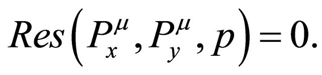
In this paper, we show that it is also possible to detect improper parameterization using the concept of Gröbner bases. We use a necessary and sufficient condition, i.e. the resultant must equal zero [13] to reveal the existence of a common Gröbner basis in a system of polynomials.
The remainder of this paper is organized as follows: Section 2 presents our algorithm for the detection of an improper parameterization. Section 3 reviews a numerical example [2]. Analysis of our algorithm is given in Section 4, and the last section concludes the work.
2. Algorithm for Detecting an Improperly Parameterized Rational Curve
In this section, we introduce our algorithm. First of all we would like to describe the definition and notation of some of the mostly used terms in this paper.
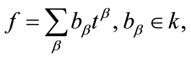
Definition 2.1: If a polynomial f in  with coefficients in k is a linear combination of monomials, then the polynomial f can be written in the form
where the summation is taken over a finite number of n-tuples , where
  are nonnegative integers. This set of polynomials in
  with coefficients in k is denoted as
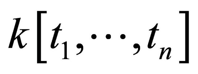 .
.
Thus, polynomials in one, two and three variables lie in ,
,  and
and , respectively. Therefore,
  denotes a field in n-variables and a field with one variable
  is normally denoted by k.
Definition 2.2: An ideal is a subset  which satisfies the following:
1) 2) If
2) If , then
 , and 3) If
  and
and , then
 .
.
Definition 2.3: Let  be polynomials in
  and let the subset I be an ideal. Then I can be written in the form

Definition 2.4: Let  denote a nonzero polynomial.
1) By letting ,
,  and
and 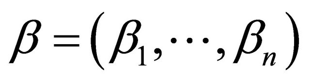 where
where 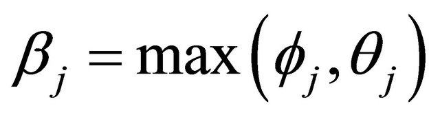 for every j; then
  is called the least common multiple of
  and
and , written in the form
 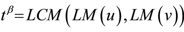 , where
  and
and  are the leading monomials of u and v respectively and
 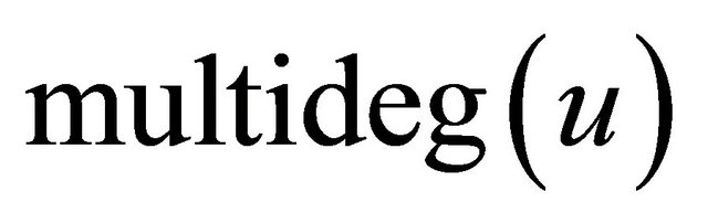 and
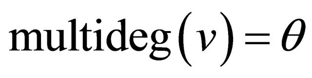
and 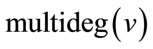 are the multidegrees of u and v respectively.
2) The S-polynomial of u and v is the combination
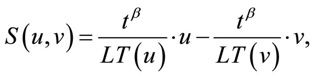
where  and
and 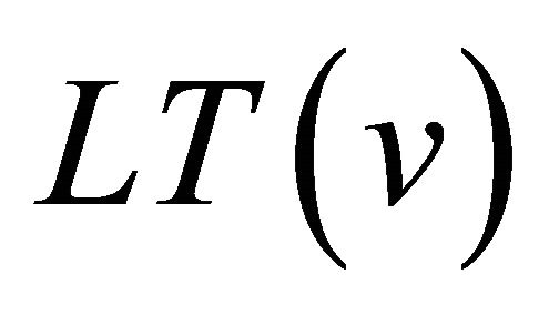 are the leading terms of u and v respectively.
Definition 2.5:  is defined as the remainder on division of
  by the ordered s-tuple .
Corollary 2.1: Suppose  are polynomials both of positive degrees, then f and g are said to have a common Gröbner basis if and only if
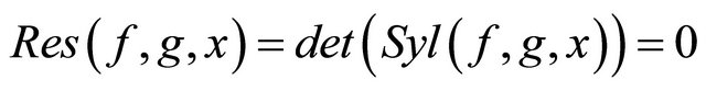
where 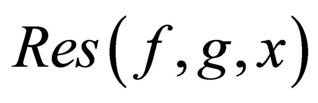 denotes the resultant of f and g with respect to x and
 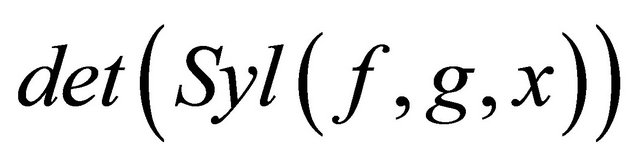 denotes the determinant of the Sylvester matrix of f and g with respect to x ([10] p. 157, Proposition 8).
Corollary 2.2: Given a Gröbner basis  of an ideal
 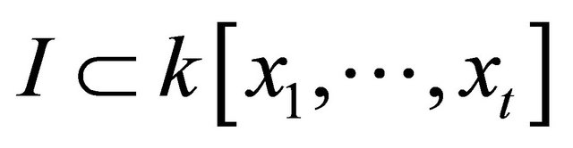 or
or , if
, if  is any polynomial and
 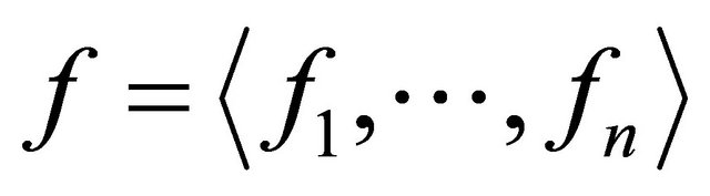 ,then the following statements are true
where  is a constant for
 , and
, and  ([10] p. 76, Theorem 4).
Given a plane rational curve of the form
 (1)
(1)
It is well known from Luroth’s theorem [14] that if Equation (1) is improperly parameterized i.e. does not give a one-to-one correspondence between the initial curve and the reparameterized curve, it is possible to reparameterize it to a properly parameterized rational curve of the form
 (2)
(2)
where
 (3)
(3)
If a nonsingular point  exists, then
 (4)
(4)
for some .
.
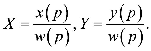
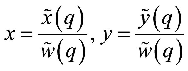
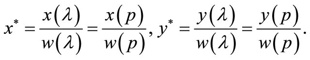
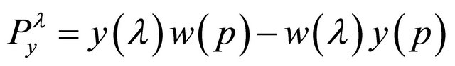
We let  and
and  where p is a parameter value of a nonsingular point on the curve, and determine the values of p that might describe the same point
 , if it exists, by developing the system of equations below
 (5)
(5)
From Equation (5), we obtain the two equations below.
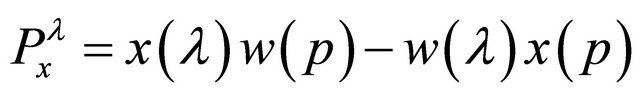 (6)
(6)
 (7)
(7)
Clearly,  and
and  are polynomials in p and if Equation (5) is true then, Equations (6) and (7) should have a common Gröbner basis which can be written (Corollary 2.1) as
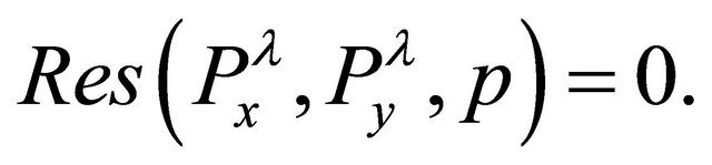 (8)
(8)
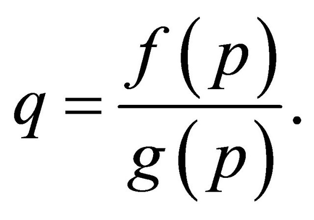
By changing the value of  to
to , in Equation (8) we obtain another equation of the form
 (9)
(9)
which implies that there are two polynomials:  and
and  with a common Gröbner basis.
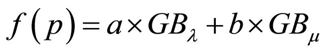
If Equations (8) and (9) hold, our next task is to evaluate the common Gröbner basis (Corollary 2.2). Let  denote the common Gröbner basis for
  and
and , and
, and  denotes the common Gröbner basis for
  and
and ; and according to Corollary 2.2, we will represent
  and
and  as
as  and
and  respectively and also represent the Gröbner basis
  and
and  as
as  and
and  respectively and hence we can write:
 (10)
(10)
 (11)
(11)
Equation (3) can be evaluated using Equations (10) and (11), while the values of a, b, c and d must be determined by using the conditions: when ,
,  and when
 ,
,  since the endpoint interpolation property must be satisfied by both curves i.e. the properly and improperly parameterized curves.
After obtaining  and
and  our final task is to determine the coefficients of Equation (2) i.e. the properly parameterized rational curve. Let
  and
and  have a maximum degree m, and u be the degree of the improperly parameterized rational curve. Hence, the degree of the properly parameterized curve shall be
 .
.
Finally; Equation (2) takes the form
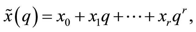 (12)
(12)
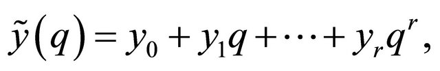 (13)
(13)
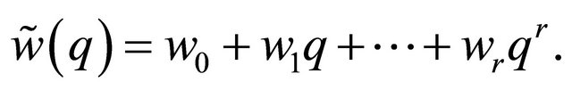 (14)
(14)
We now use the method of undetermined coefficients [15] to find the coefficients ,
,  , and
, and .
.
The whole algorithm is summarized as follows:
1) At the beginning we pick  values of p.
2) We follow the procedures above and compute .
.
a) If  gives a one-to-one relationship between q and p (i.e. properly parameterized) the algorithm will CONTINUE by selecting a new value of p from step 1.
b) If  doesn’t give a one-to-one relationship between q and p (i.e. improperly parameterized) the algorithm will TERMINATE.
Our algorithm will not terminate at step 2(a) iff the equation  gives a one-to-one relationship between q and p i.e. properly parameterized; but will terminate at step 2(b) if
  does not give a oneto-one correspondence between q and p i.e. improperly parameterized.
In this paragraph, we would throw light on how the Gröbner basis of an ideal is computed using Buchberger’s algorithm ([10] p. 90, Theorem 2). The uniqueness of the Buchberger algorithm in this paper is that, it gives not only Gröbner basis as is usual but a common Gröbner basis when applied to a  field. Given a polynomial ideal
 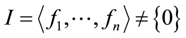 then, the algorithm proceeds as follows:
Input: 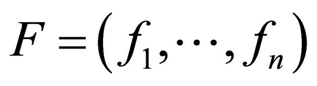
Output: a Gröbner basis  for I, with
REPEAT
FOR each pair ,
,  in
in  DO
DO

IF  THEN
THEN
UNTIL 
At the initial phase of the algorithm, G is enlarge by adding the remainder  for
for . If
. If
 , then u, v and
  are also in I and therefore, since we are dividing by
 , we obtain
 . It is interesting to note that G contains the given basis F of I and as such, G is a real basis of I. The algorithm terminates when
 , which means that
for .
.
Finally, it is necessary to note that if the polynomial ideal I is in the  field, then the above algorithm will give only one Gröbner basis (i.e. common Gröbner basis) that is common to both ideal members.
3. Review of a Numerical Example
In this section we solve a numerical example from [2] using our algorithm to detect improper parameterization.
We consider the rational cubic Bezier curve defined by the equations
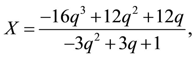
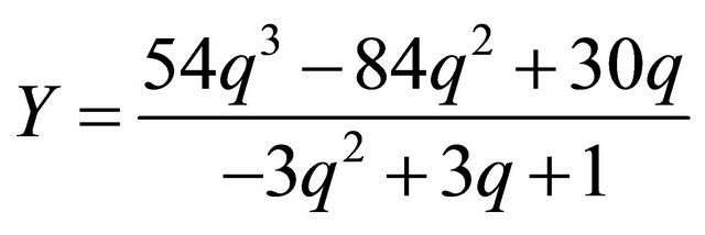
and compute the parametric substitution that gives the equations below
We pick  and
and . When
 , we have:
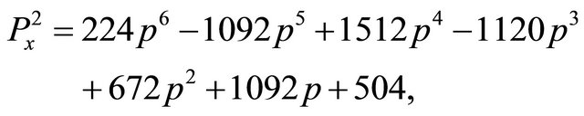

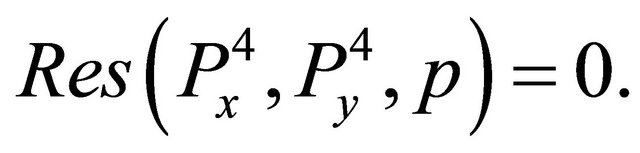
The resultant of these two polynomials is:

This means that 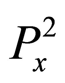 and
and 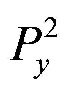 have a common Gröbner basis
 . Therefore, the
  of these two polynomials is:

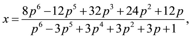
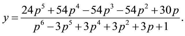
When , we have:

The resultant of  and
and  is:
is:
This tells us that there is a common Gröbner basis for the two polynomials. Hence, GB4 for the two polynomials is:

Our parametric substitution becomes

We now use the endpoint interpolation property i.e.  when
when  and
and  when
when  and determine a, b, c and d to compute our parameter. The first condition gives
 , and then select
 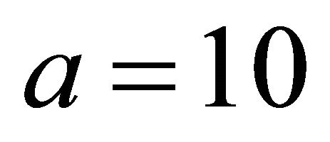 and
and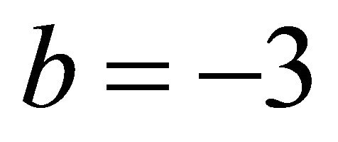 . The second constraint gives
 , we choose
 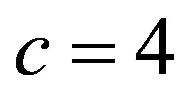 and
and , and finally obtain our parameter
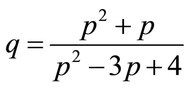 .
.
4. Analysis
In [2], the algorithm uses an assumption for the existence of a common factor for the two polynomials and finally compute this common factor using the concept of the Euclidean algorithm.
In this piece of work, we utilize a necessary and sufficient condition to confirm that the two polynomials have a common Gröbner basis.In Section 3, we see that the existence of common Gröbner basis for both values 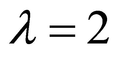 and
and 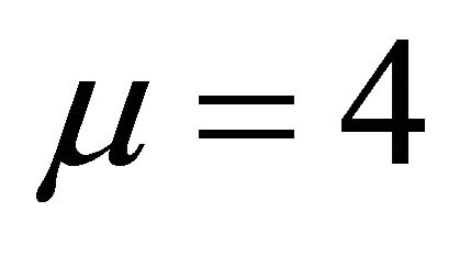 is confirmed by the fact that both
 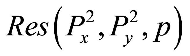 and
and 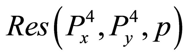 equals zero. After confirming the existence of a common Gröbner basis the algorithm is then used to compute this common Gröbner basis.
From Section 3, we see also that there is a one-to-two correspondence between parameter values of q and p, i.e. one value of q gives two values of p as it is evident from the obtained parametric relation ; and also the parameterization has a tracing index of two i.e. the curve is doubly traced.Therefore, the curve is improperly parameterized.
5. Conclusions
The algorithm in [2] assumes that there is a common factor for the two polynomials and then uses the notion of the Euclidean algorithm to compute the common factor. However, it is interesting to note that the Euclidean algorithm requires divisibility in the field  [10]. Our algorithm, first of all, confirms the existence of a common Gröbner basis before any computational attempt is made.
The advantages of our algorithm are as follows: Our algorithm always confirms the existence of a common Gröbner basis before computation. Secondly, it is based on the concepts of Gröbner bases, which requires operations in the field . We just need to indicate the ordering i.e. lexicographic order, graded lexicographic order, or graded reverse lexicographic order.
Finally, from our algorithm in Section 2, we conclude with no doubt that it is also possible to detect improper parameterization using the notion of Gröbner bases iff the polynomial ideal I is in the  field.
6. Acknowledgements
The authors would like to thank the anonymous referees for their useful comments on this paper. We would also like to thank the Chinese Scholarship Council.
REFERENCES
- D. Manocha and J. F. Canny, “Rational Curves with Polynomial Parameterization,” Computer-Aided Design, Vol. 23, No. 9, 1991, pp. 645-652. doi:10.1016/0010-4485(91)90042-U
- T. W. Sederberg, “Improperly Parametrized Rational Curves,” Computer Aided Geometric Design, Vol. 3, No. 1, 1986, pp. 67-75. doi:10.1016/0167-8396(86)90025-7
- M. V. Hoeij, “Rational Parametrizations of Algebraic Curves Using a Canonical Divisor,” Journal of Symbolic Computation, Vol. 23, No. 2-3, 1997, pp. 209-227. doi:10.1006/jsco.1996.0084
- T. Recio and J. R. Sendra, “Real Parametrizations of Real Curves,” Journal of Symbolic Computation, Vol. 23, No. 2-3, 1997, pp. 241-254. doi:10.1006/jsco.1996.0086
- J. R. Sendra and F. Winkler, “Parameterization of Algebraic Curves over Optimal Field Extensions,” Journal of Symbolic Computation, Vol. 11, 2008, p. 1-000.
- J. R. Sendra and F. Winkler, “Symbolic Parameterization of Curves,” Journal of Symbolic Computation, Vol. 12, No. 6, 1991, pp. 607-631.
- J. R. Sendra and F. Winkler, “Tracing Index of Rational Curve Parameterizations”. www.risc.jku.at/publications/download/risc_264/Nr.17_final-1.pdf
- G. Salmon, “Higher Plane Curves,” G.E. Stechert and Co., New York, 1879, 30 p.
- R. J. Walker, “Algebraic Curves,” Princeton, 1950, 67 p.
- D. A. Cox, J. Little and D. O’Shea, “Ideals, Varieties and Algorithms,” Introduction to Computational Algebraic Geometry and Commutative Algebra, 2nd Edition, Springer, Berlin, 1991, pp. 49-168.
- H. Hong and J. Schicho, “Algorithms for Trigonometric Curves (Simplification, Implicitization and Parameterization),” Technical Report, 1997. http://www.risc.uni-linz/people/hhong-jschicho
- J. Harris, “Graduate Texts in Mathematics,” Algebraic Geometry: A First Course, Springer-Verlag, Berlin, 1992, pp. 3-16.
- L. Buse and T. L. Ba, “Matrix-Based Implicit Representation of Rational Algebraic Curves and Applications,” Computer Aided Geometric Design, Vol. 27, No. 9, 2010, pp. 681-699. doi:10.1016/j.cagd.2010.09.006
- J. W. Archbold, “Introduction to the Algebraic Geometry of a Plane,” Edward Arnold & Co., London, 1948.
- J. Li, “General Explicit Difference Formulas for Numerical Differentiation,” Journal of Computational and Applied Mathematics, Vol. 183, No. 1, 2005, pp. 29-52. doi:10.1016/j.cam.2004.12.026
NOTES
*Corresponding author.