American Journal of Computational Mathematics
Vol.2 No.2(2012), Article ID:20092,4 pages DOI:10.4236/ajcm.2012.22015
A Wavelet Based Method for the Solution of Fredholm Integral Equations
Central Michigan University, Mount Pleasant, USA
Email: enbing.lin@cmich.edu
Received December 20, 2011; revised January 17, 2012; accepted January 26, 2012
Keywords: Coiflet; Scaling Function Interpolation; Wavelet; Fredholm Integral Equation; Multiresolution Analysis
ABSTRACT
In this article, we use scaling function interpolation method to solve linear Fredholm integral equations, and we prove a convergence theorem for the solution of Fredholm integral equations. We present two examples which have better results than others.
1. Introduction
Integral equations play an important role in both mathematics and other applicable areas. Many physical phenomena can be modeled by differential equations. In fact, a differential equation can be replaced by an integral equation that incorporates its boundary conditions. Integral equations are also useful in many branches of pure mathematics as well. Here we study Fredholm integral equations [1-3].
Wavelets have been applied in a wide range of engineering and physicaldisciplines, and it is an exciting tool for mathematicians. In this paper we will find a numerical solution for the second kind Fredholm integral equation of the form
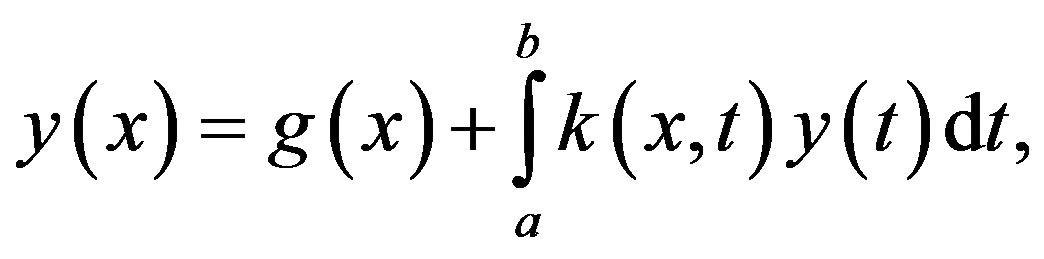 (1)
(1)
where the function  and are
  given, and the unknown function
  is to be determined.
1.1. Wavelets
In this subsection we will provide a brief account of wavelet transform and Multiresolution analysis (MRA). We first define the scaling function  and the sequence
  such that
 (2)
(2)
By using this dilation and translation [4], we defined a nested sequence spaces  which is called MRA of
  with the following properties
 (3)
(3)
 (4)
(4)
 is dense in
 (5)
(5)
 (6)
(6)
For the subspace  is built by
 then
then  and since
  we can write
In general,
 (7)
(7)
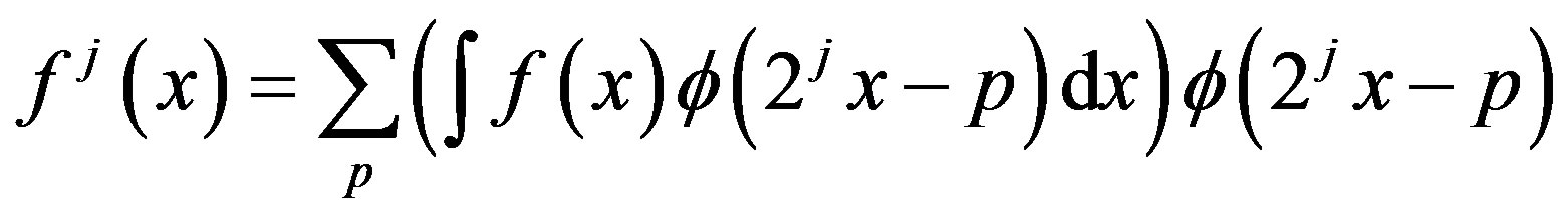
Any function  can be approximated by scaling functions in one of the subspace in the given nested sequence. In fact, for each j we define the orthogonal complement subspace
  of
of  in the subspace
 . The orthogonal basis of
  is denoted by
 (8)
(8)
and the wavelet function can be obtained by
 . (9)
. (9)
Some interesting properties of scaling and wavelet functions make wavelet method more efficiently than quadrature formula methods and spline approximations in solving Integral equations. A lot of computational time and storage capacity can be saved since we do not require a huge number of arithmetic operations partly due to the following properties.
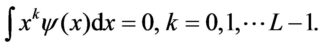
1) Vanishing Moments:
 (10)
(10)
and in this case the wavelet is said to have a vanishing moments of order m2) Semiorthogonality:
 (11)
(11)
The set of scaling functions  are orthogonal at the same level n, which means:
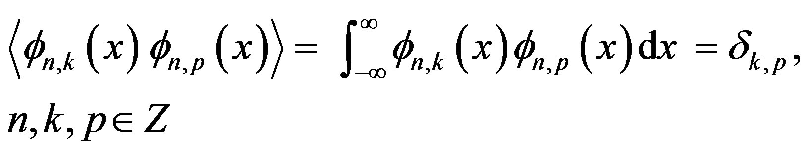 (12)
(12)
Coiflet (of order L) has more symmetries and is an orthogonal multiresolution wavelet system with,
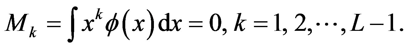 (13)
(13)
 (14)
(14)
where  are the moments of the scaling functions.
1.2. Scaling Function Interpolation
The function  can be interpolated by using the basis functions in the subspace
  as follows.
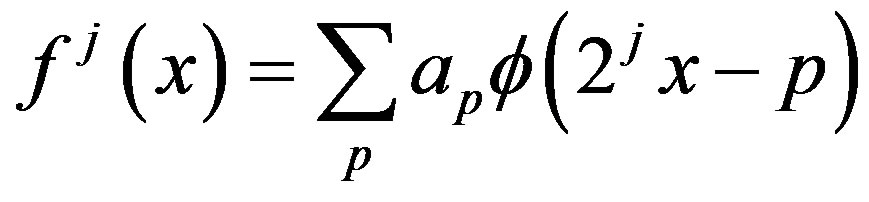 (15)
(15)
where  are the coefficients evaluated by using equation (12) such that
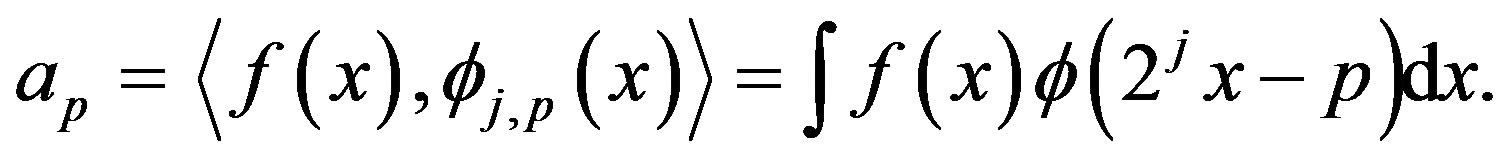 (16)
(16)
Hence the equation (15) becomes:
 .
.
On the other hand, one can use sampling values of  at certain points to approximate the function
  It is proved in [5], namely, an interpolation theoremusing coiflet such that if
  and
and  are sufficiently smooth and satisfy the equations (10)-(14) and the function
 , where
  is a bounded open set in
Then,
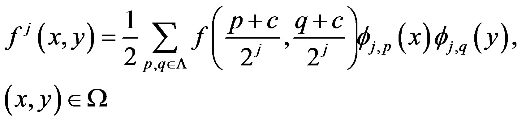 (17)
(17)
where the index set is
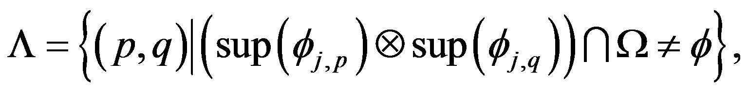
Sup denote the support of a function.
In addition, the moment  satisfies
Then,
where  is a constant depending only on
 , diameter of
  and
and
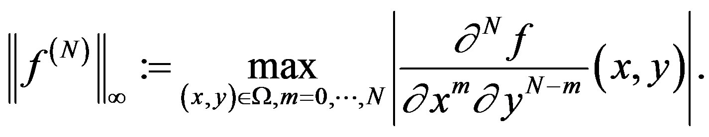
For the function with one variable, we have
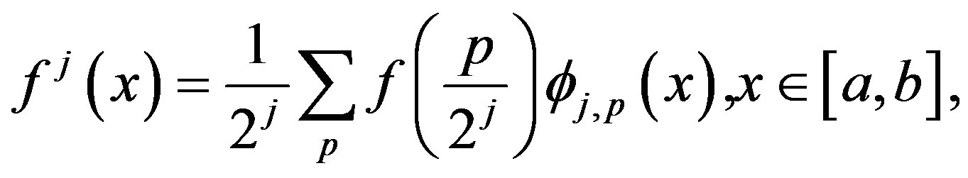 (18)
(18)
and
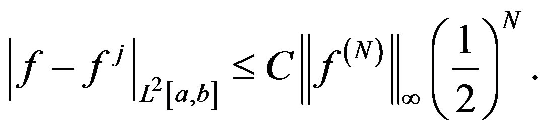 (19)
(19)
where
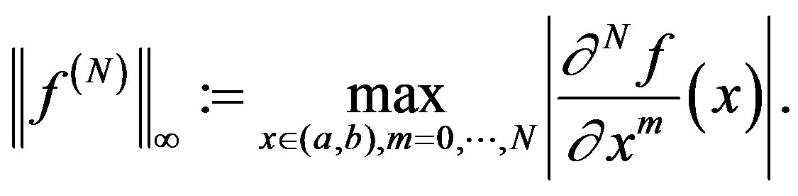 (20)
(20)
2. Solve Fredholm Integral Equations Using Coiflet
In this section we will apply coiflet and the interpolation formula (18) to solve the Fredholm integral equation (1). The unknown function  in equation (1) can be expanded in term of the scaling functions
  in the subspace
  such that
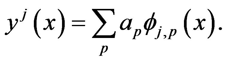 (21)
(21)
Consider the equation (1) and the function  which is defined on the interval [a, b] and the scaling function
  defined on the interval
  then we have the index:
By applying equation (21) into equation (1), we get the system,
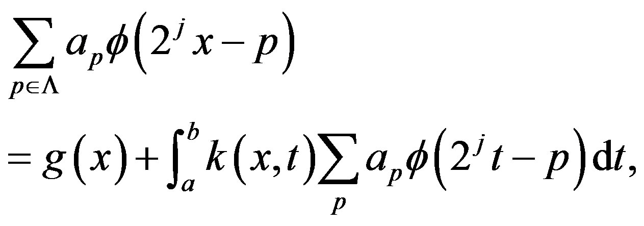 (22)
(22)
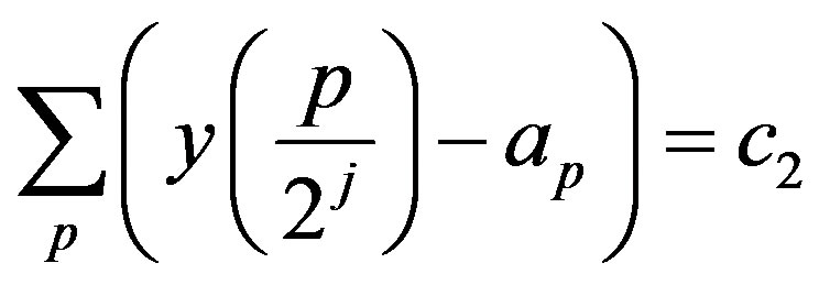
which is equivalent to the following system,
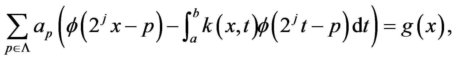 (23)
(23)
where thecoefficients  can be evaluated by substituting
  into the system (23). Moreover, the system (23) can be expressed in compact form,
 (24)
(24)
where
Then 
This gives rise to coefficients in (21) and we obtain a numerical solution of (1). In what follows, we will derive a convergence theorem of this numerical solution.
3. Error Analysis
In this section will discuss the convergence rate of our method for solving linear Fredholm integral equation (1).
Theorem 1. In equation (1), supposethat the function  and the functions
  and
and , for
, for 
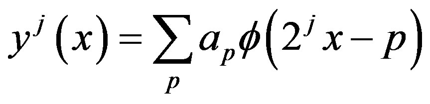 (25)
(25)
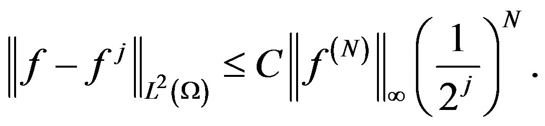
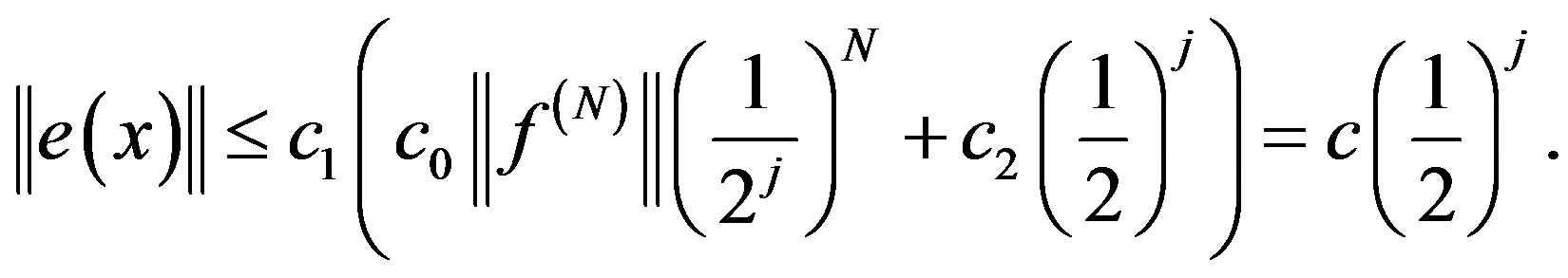
is an approximate solution of the equation (1) with the coefficients obtained in (24). Then,
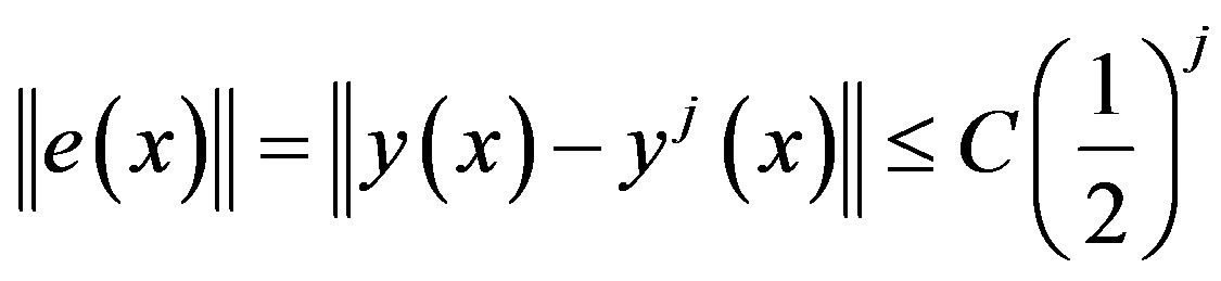 (26)
(26)
where,
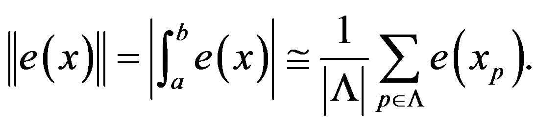
Proof. Subtracting equation (25) from equation (1) and taking the norm for both sides, we get the following
 (27)
(27)
where 
By [5], the unknown function  can be interpolated by using coiflet such that:
 (28)
(28)
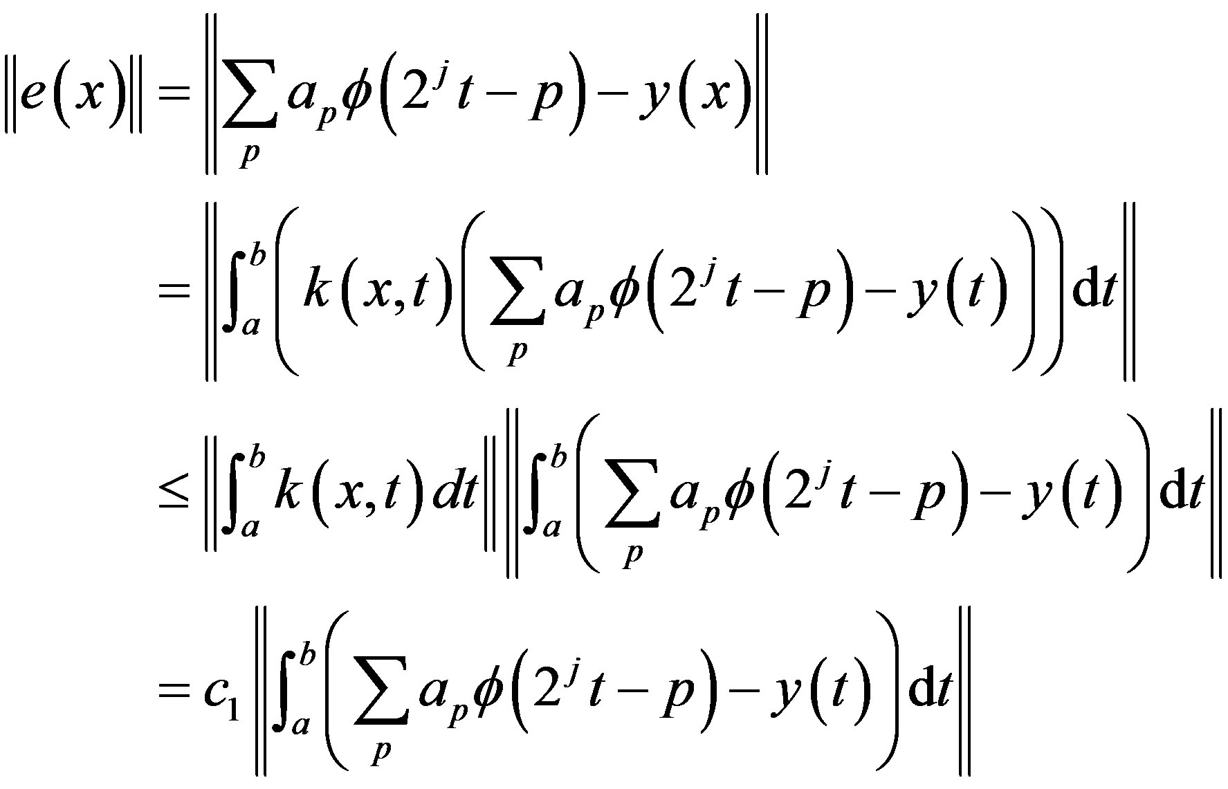
Let  in equation (28) then add and subtract it in equation (27), we get the following inequalities.
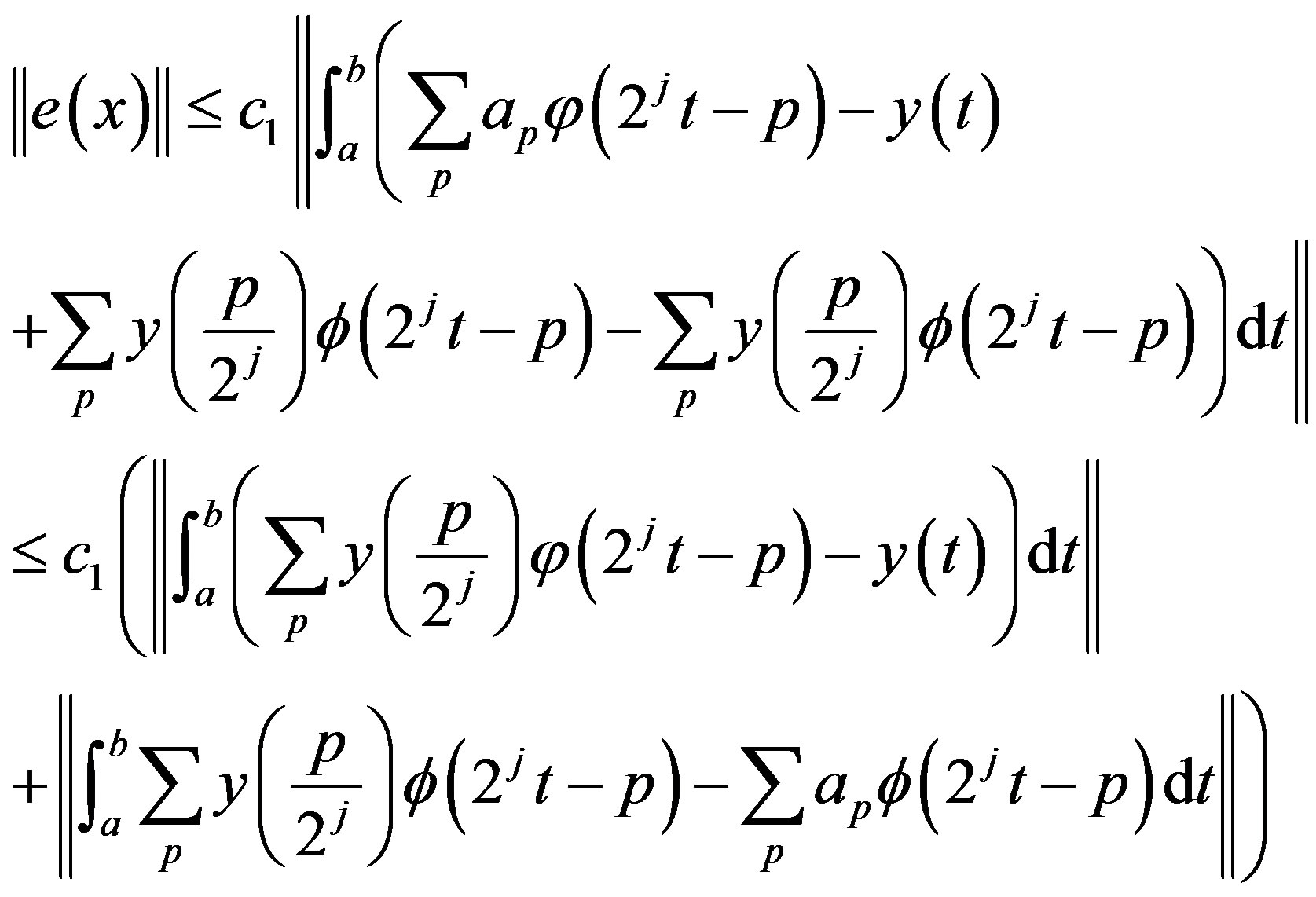
which equals to the equation
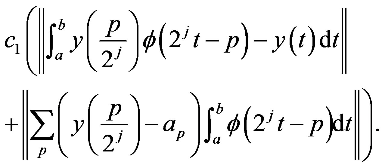 (29)
(29)
By [5], we have
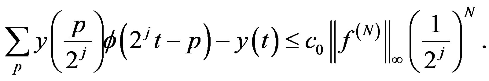 (30)
(30)
Since 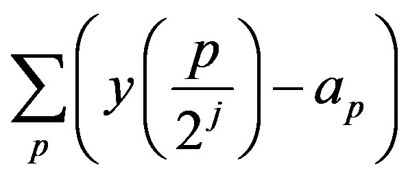 is finite we define it as
 . (31)
Using the above results and the orthonomality of the scaling functions , we conclude that
 (32)
(32)
4. Numerical Examples
In the following examples, we will solve linear Fredholm integral equation (1) using coiflet of order 5 and provide errors between exact solutions and our numerical solutions at different resolution levels. Both examples are also presented in [6] by using different method.
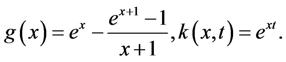
Example 1.
Consider 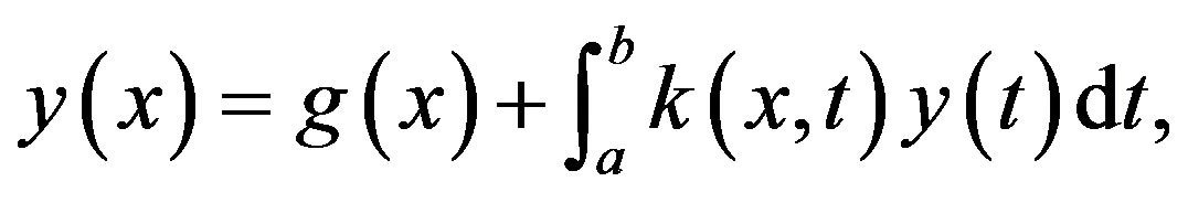 where
where
The exact solution is  and
and 
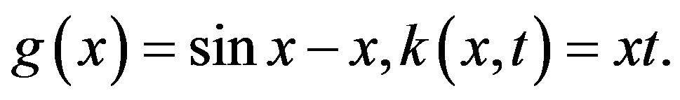
Example 2.
Consider

where  and
and  are given on the interval [0,1] such that,
The exact solution is 
We use our interpolation method to solve the above integral equations, and find the errors in Table 1.
5. Conclusion
In this work, we use our interpolation method by using coiflets to solve Fredholm integral equations, and compare our results with those in [6]. It turns out our method is more efficient with better accuracy. Moreover, our method can be applied to different kind of integral equations as well as integral-algebraic equations. Although the results in the above examples don’t seem to have
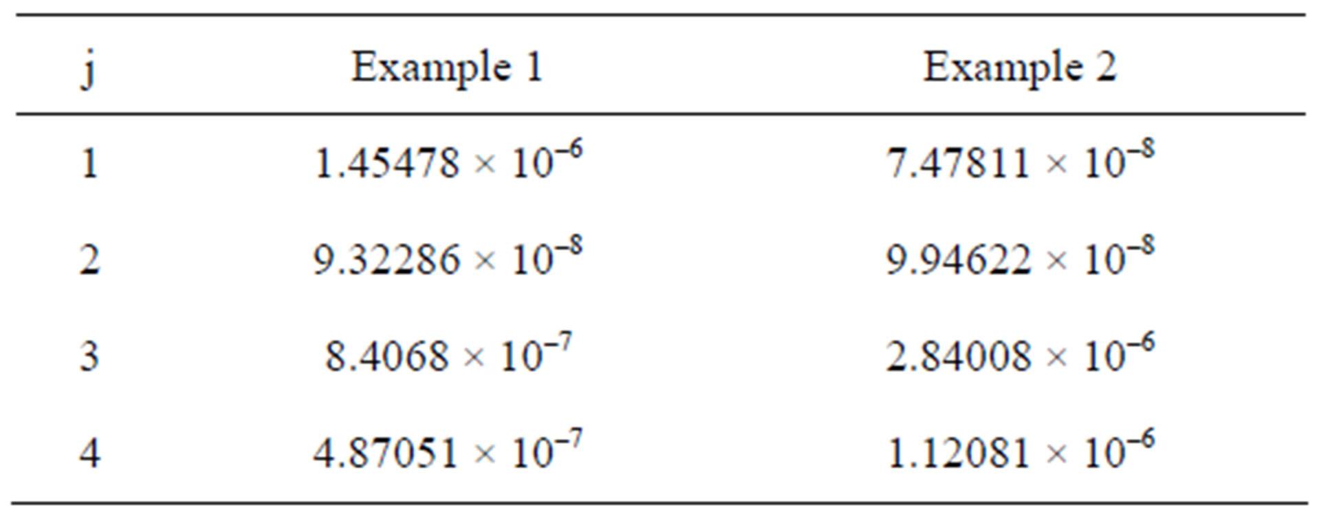
Table 1. The error e(x) for examples 1 and 2 with different values of j.
correlation with the level of resolutions but they basically validate our theorem. In fact, we can also interpolate the given functions in the integral equation. This would simplify the calculations in finding numerical solutions of integral equations. It would be interesting to use our method to solve nonlinear integral equations as well.
6. Acknowledgements
The authors would like to thank the anonymous referees for their helpful comments.
REFERENCES
- F. Brauer, “On a nonlinear Integral Equation for Population Growth Problems,” SIAM Journal on Mathematical Analysis, No. 6, 1975, pp. 312-317.
- F. Brauer and C. Castillo, “Mathematical Models in Population Biology and Epidemiology,” Springer-Verlang, New York, 2001.
- T. A. Butorn, “Volterra Integral and differential equations,” Academic Press, New York, 1983.
- K. C. Charles, “In Introduction to Wavelets,” Academic Press, New York, 1992.
- E. B. Lin and X. Zhou, “Coiflet Interpolation and Approximate Solutions of Elliptic Partial Differential Equations,” Numerical methods for Partial Differential Equations, Vol. 13, No. 4, 1997, pp. 302-320. doi:10.1002/(SICI)1098-2426(199707)13:4<303::AID-NUM1>3.0.CO;2-P
- K. Maleknjaf and T. Lotfi, “Using Wavelet For Numerical Solution of Fredholm Integral Equations,” Proceedings of the World Congress on Engineering, London, 2-4 July 2007, pp. 2-6.