American Journal of Operations Research
Vol. 3 No. 3 (2013) , Article ID: 31679 , 7 pages DOI:10.4236/ajor.2013.33035
Computing the Distribution Function of the Number of Renewals
Department of Mathematics and Computer Science, Royal Military College of Canada, Kingston, Canada
Email: chaudhry-ml@rmc.ca, xiaofeng.yang@rmc.ca, ong-b@rmc.ca
Copyright © 2013 Mohan L. Chaudhry et al. This is an open access article distributed under the Creative Commons Attribution License, which permits unrestricted use, distribution, and reproduction in any medium, provided the original work is properly cited.
Received April 20, 2013; revised May 25, 2013; accepted June 15, 2013
Keywords: Number of Renewals; Rational Approximation; Padé
ABSTRACT
The method of Laplace transforms is used to find the distribution function, mean, and variance of the number of renewals of a renewal process whose inter-arrival time distribution has a rational Laplace transform. Where the Laplace transform is not rational, we use the Padé approximation method. We apply our method to certain examples and the results are compared to those reported by other researchers.
1. Introduction
Renewal and reliability theories are powerful modeling tools in many applications, considering, for example, a series of renewals during a time interval  with the inter-renewal times having certain distributions. The interest, usually, is to find the distribution or the moments of the number of renewals during the interval
 . Although the theoretical aspects of renewal theory have been discussed in various books such as Cox [1] and Feller [2,3], not much seem to have been done in applying the theoretical results to practice for lack of availability of easily computable results. Using the cubic splining algorithm to compute the recursively-defined convolution integrals that appear in renewal theory, Baxter et al. [4] is able to construct some tables for the mean and variance of the number of renewals for different inter-renewal time distributions with varying parameters. A straightforward method to compute the convolution integral is to use the Laplace transform (LT) method. Using the root-finding method, Chaudhry [5] develops a unified method to compute the mean and variance of the number of renewals. Though the means and variances are useful for many applications, this paper goes a step further and deals with computing the distribution of the number of renewals from which one can get more information than from the mean and variance.
There are several methods that can be used for the numerical inversion of generating functions (GFs); see the excellent reviews on the numerical inversion (of GFs as well as of LTs) by Abate et al. [6-9]. Some researchers have been critical of using the method of roots, see, e.g. Cox and Smith [10] and Kleinrock [11]. In view of this, this paper serves another useful purpose and shows that with the availability of high precision in current software packages, the roots can be found successfully and used to invert the transforms. Further, using the roots method, the results can be first given in an analytically explicit form and then used to find the final results.
2. Theory
2.1. Problem Description and Method of Laplace Transforms
Let  be a governing sequence of independently identically distributed (i.i.d.) inter-renewal times for the renewal process
 , where
  denotes the number of renewals in
 . Let
. Let  represent the generic inter-renewal time with cumulative distribution function (CDF)

and probability density function (pdf) .
.
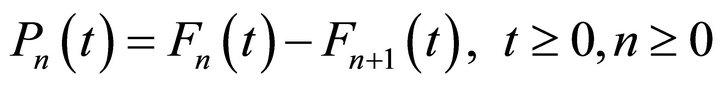
Define the probability mass function (pmf)
 . Let
. Let
 . For
. For ,
,  represents the time when the n-th renewal occurs. Define
  , with
 . Then

is the n-fold convolution of  with itself, and (see Chaudhry and Templeton [12])
 (1)
(1)
Let  and
and  be the Laplace-Stieltjes transform (LST) of
  and
and , respectively, defined by
 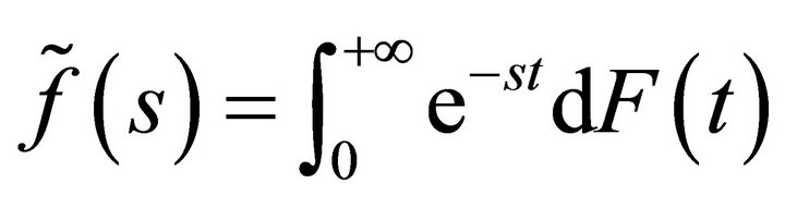 and
and .
.
Taking the LST on both sides of Equation (1), we get
 (2)
(2)
and hence
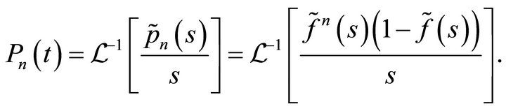 (3)
(3)
2.2. Inversion of Laplace Transforms
2.2.1.  Is a Rational Function
The inverse LT Equation (3) can be obtained analytically using partial fractions. Let
where  and
and  are polynomials of degree
  and at most
 , respectively. Then by Equation (2), we have
 (4)
(4)
which is a rational function.
Without loss of generality, we assume that the equation  has
has  distinct roots
 . Since
 ,
,  and
and  have the same constant terms,
 . And Equation (4) can be expressed in partial fractions as

where the constant coefficient  is given by
The final inversion can be written as
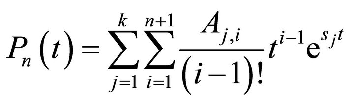 (5)
(5)
The case when  has repeated roots can be dealt with similarly.
2.2.2.  Is Not a Rational Function
We use the Padé approximation method. Assume
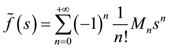
where
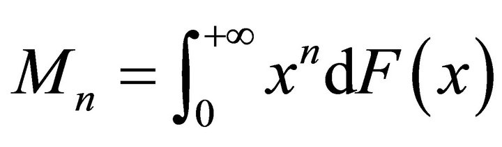
is the n-th moment of the inter-renewal time. We can find a rational approximation function
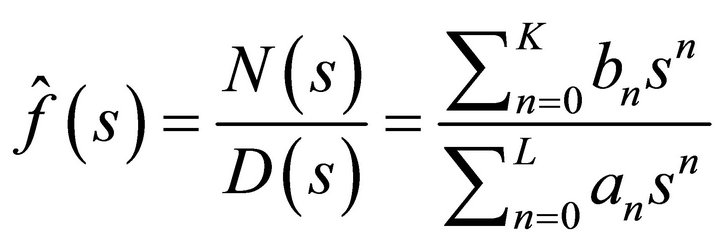
where  and
and  are polynomials of degree
  and
and![]() , respectively with undetermined coefficients
, respectively with undetermined coefficients  and
and , such that the first
  moments of
  are equal to those of
 . We denote the above Padé approximation as
  (Baker et al. [13]). In practice,
  is set to one and
  and
and ![]() are chosen by trial and error. Equating the moments and formulating the simultaneous equations, the coefficients bn and an are uniquely determined (Baker et al. [13], Harris [14]).
are chosen by trial and error. Equating the moments and formulating the simultaneous equations, the coefficients bn and an are uniquely determined (Baker et al. [13], Harris [14]).
Use of continued fractions is another way to obtain an approximate rational function . The method is, in fact, a special case of the Padé method (Baker et al. [13]).
There are times when using Padé method directly is not possible or does not give the desired results. For example, the Pareto distribution has an infinite second moment, and directly equating the moments cannot be done. For the lognormal distribution, the waveform of the Padé approximated distribution function shows quite large errors. The solution is to have a two-step approximation. The first step is to use line segments to approximate the distribution function. In the second step, the Padé method is used to generate a rational LT. By adjusting the parameters in these two steps,  can be obtained with the desired properties. We will illustrate this technique in the examples.
2.3. Verification of the Distribution
The expected number of renewals of  in
in  is given by
and its variance by
In all our examples, the  obtained in Equation
(5) is used to compute  and
and , and are checked against the results obtained by (Chaudhry [5]) using

and

In addition, we also match the resulting mean and variance with those of Baxter et al. [4].
3. Examples
3.1. Erlang Distribution
We first consider the simple case where  follows the Erlang distribution with the shape parameter equal to 2, and we can get exact analytical results.
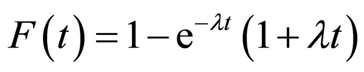
The pdf and CDF of  are given, respectively, by

and
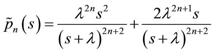
Thus,

We get

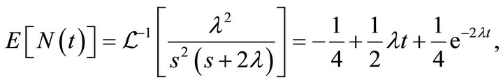
and
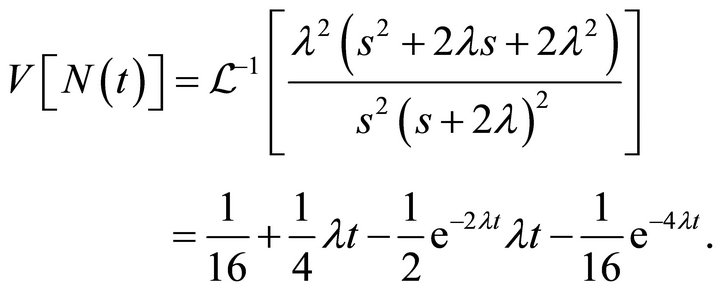
It may be remarked that the analytic expression for the mean has been incorrectly reported by Parzen [15, p. 177].
3.2. Mixed Generalized Erlang Distribution
The pdf and LST of a Mixed Generalized Erlang (MGE) distribution are given, respectively, by
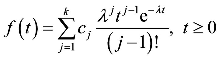
and

with 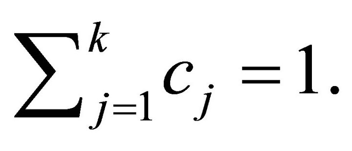 We consider the case of MGE with
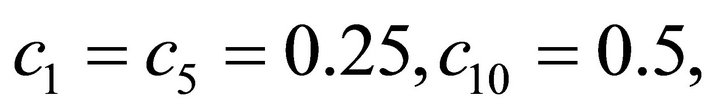 and
and  The
The , mean and variance are obtained by the LT method discussed in Section 2.2. Table 1 shows the results for several values of
 . They are checked against the known results obtained without using roots by Chaudhry [5].
The graph in Figure 1 shows that the  calculated from the obtained distribution functions asymptotically converges to the line
 (6)
(6)
derived in [16], where  and
and  are the first and
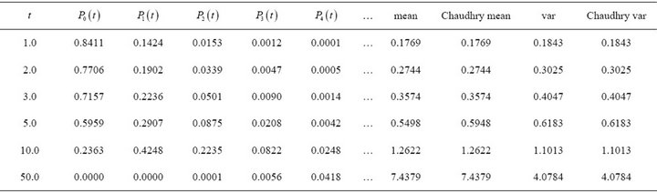
Table 1.  for MGE distribution with
  and
and .
.
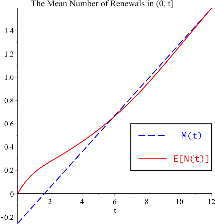
Figure 1.  asymptotically converges to the line
second moments of . As expected, one can see from this graph that the results given in Equation (6) are good only for large t.
3.3. Matrix Exponential Distribution
Consider the matrix exponential and non-phase-type distribution (see Bladt [17]) given below. The pdf and its LT are, respectively,

and
Using partial fractions for transform inversion, we obtain  for some selected
  values. The results are listed in Table 2.
3.4. Gamma Distribution
The pdf and LST of the Gamma distribution are given, respectively, by
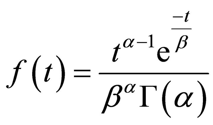
and

where ![]() and
and  are the shape and scale parameters, respectively. In this example, we set
  and α = 0.55. The Padé [4/5] approximation of
  is given by

The  are obtained and some selected pmf's, means, and variances are tabulated together with those from Baxter et al. [4] in Table 3.
3.5. Weibull Distribution
The pdf
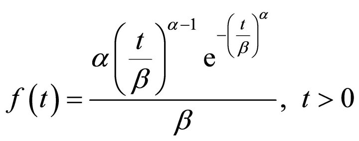
and the CDF
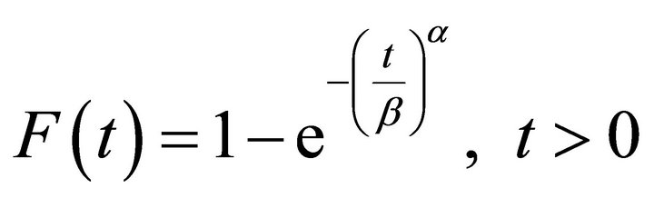
of the Weibull distribution do not have the closed-form LT. However, the moments of the Weibull distribution can be obtained from its CDF to use in the Padé method. For  and
and , we equate moments up to the 8-th moment in the Padé [2/6] approximation, and get

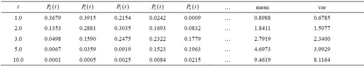
Table 2.  for the non-phase-type distribution discussed in Section 3.3.
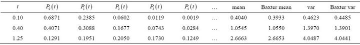
Table 3.  for the Gamma distribution with
  and
and .
.
Some selected results are listed in Table 4 together with Baxter’s (see Baxter et al. [4]). It is noted that when t becomes large, our resulting means and variances match those of Chaudhry [5].
3.6. Truncated Normal Distribution
The pdf of the truncated normal distribution is given by
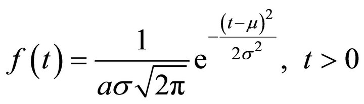
where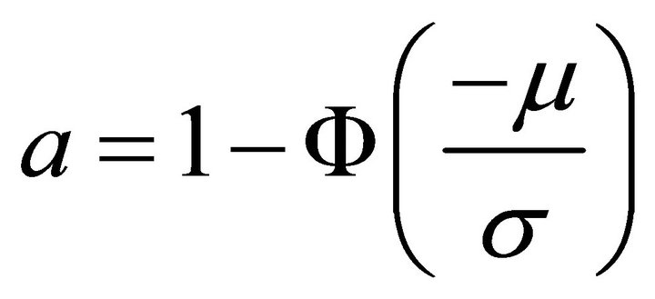 , with
  being the standard normal distribution function. By the Padé [5/6] approximation

we are able to obtain . Some results and comparisons are shown in Table 5.
3.7. Inverse Gaussian Distribution
The pdf for the inverse Guassian distribution is
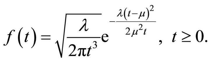
Setting  and
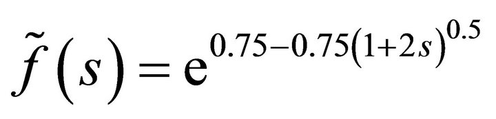
and , its LST is given by
where ![]() and
and  can also be expressed in terms of the shape and scale parameters
  and
and , respectively, (see Baxter et al. [4]). By the Padé [4/7] approximation, we get

Some results are shown in Table 6 along with the results of Baxter et al. [4].
3.8. Lognormal Distribution
The pdf

and CDF
of the lognormal distribution have no closed-form LT. Using the Padé approximation method directly on the lognormal distribution does not lead to the desired results. Our solution is a two-step approximation. In the first step, we sample uniformly N points of , and then connect the adjacent points to form
  line segments as the first approximation of the lognormal distribution. The
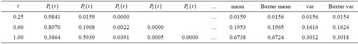
Table 4.  for the Weibull distribution with
  and
and .
.

Table 5.  for the Truncated Normal distribution with
  and
and .
.
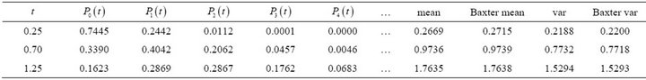
Table 6.  for the Inverse Gaussian distribution with
  and
and .
.

Table 7.  for the Lognormal distribution with
  and
and .
.
uniform sampling step size used is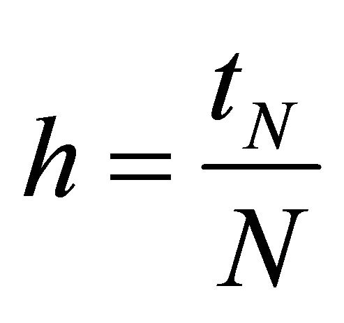 , where tN is chosen arbitrarily such that
  is close to 1. In additionthe last line segment is modified to reach 1 at tN. The resulting first approximation function can be written as
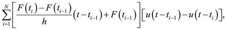
where  are unit step functions. In this example,
  is set to 0 and
  to 1. Accordingly, we set
  and
and .
.
In the second step, the LST of the first approximation function is obtained and expanded as a Taylor series. Using the Padé [7/8] method, we have the second approximation of  to be
to be

Table 7 lists selected , means and variances along with the results of Baxter et al. [4].
4. Conclusions
Using Laplace transforms, it is shown that computing the distribution of the number of renewals is straightforward when the LT of the inter-renewal time distribution is rational. For inter-renewal time distributions having nonrational LTs, the Padé method provides good approximations. For the case where the inter-renewal time distributions do not have Laplace transforms, we provide the line segment approximation for the distribution function and apply the Padé method thereafter.
The proposed numerical method is not limited to compute the distribution of number of renewals. It can be applied to other similar processes such as alternating renewal process, the superposition of renewal processes, and cumulative processes, for which Laplace transforms are used to solve such problems. Further, the method discussed here can be applied to more complex models such as bulk-renewal processes both in discreteand continuous-times once the analytic results are known.
5. Acknowledgements
The first author acknowledges with thanks for the partial support he received through NSERC #17287 for carrying out this research.
REFERENCES
- D. R. Cox, “Renewal Theory,” John Wiley & Sons Inc., New York, 1962.
- W. Feller, “Probability Theory and Its Applications Vol. II,” Wiley, New York, 1966.
- W. Feller, “An Introduction to Probability Theory and Its Applications,” Wiley, New York, 1967.
- L. A. Baxter, E. M. Scheuer, D. J. McConalogue and W. R. Blischke, “On the Tabulation of the Renewal Functions,” Technometrics, Vol. 24, No. 2, 1982, pp. 151-156. doi:10.1080/00401706.1982.10487739
- M. L. Chaudhry, “On Computations of the Mean and Variance of the Number of Renewals: A United Approach,” The Journal of the Operations Research Society, Vol. 46, 1995, pp. 1352-1364.
- J. Abate, G. L. Choudhury and W. Whitt, “A Unified Framework for Numerically Inverting Laplace Transforms,” Informs Journal on Computing, Vol. 18, No. 4, 2006, pp. 408-421. doi:10.1287/ijoc.1050.0137
- J. Abate, G. L. Choudhury and W. Whitt, “An Introduction to Numerical Transform Inversion and Its Application to Probability Models,” In: W. Grassman, Ed., Computational Probability, Kluwer, Boston, 1999, pp. 257- 323.
- J. Abate and W. Whitt, “Numerical Inversion of Laplace Transforms of Probability Distributions,” ORSA Journal on Computing, Vol. 7, No. 1, 1995, pp. 36-43. doi:10.1287/ijoc.7.1.36
- J. Abate and W. Whitt, “The Fourier-Series Method for Inverting Transforms of Probability Distributions,” Queueing Systems, Vol. 10, No. 1-2, 1992, pp. 5-88. doi:10.1007/BF01158520
- D. R. Cox and W. L. Smith, “Queues,” Methuen and CO Ltd., London, 1967.
- L. Kleinrock, “Queueing Systems Volume I: Theory,” John Wilery & Sons, New York, 1975, pp. 212-312.
- M. L. Chaudhry and J. G. C. Templeton, “A First Course on Bulk Queues,” John Wiley & Sons Inc., New York, 1983.
- G. A. Baker and P. Graves-Morris Jr., “Padé Approximants (Encyclopedia of Mathematics and Its Applications),” 2nd Edition, Cambridge University Press, Cambridge, 1996.
- C. M. Harris and W. G. Marchal, “Distribution Estimation Using Laplace Transform,” INFORMS Journal on Computing, Vol. 10, No. 4, 1998, pp. 448-458. doi:10.1287/ijoc.10.4.448
- E. Parzen, “Stochastic Processes,” Holden-Day Inc., San Francisco, 1962.
- M. L. Chaudhry and B. Fisher, “Simple and Elegantderivations for Some Asymptotic Results in the DiscreteTime Renewal Process,” Statistics and Probability Letters, Vol. 83, No. 1, 2012, pp. 408-421.
- M. Bladt, “Computational Method in Applied Probability,” Aalborg University, 1993.