Int'l J. of Communications, Network and System Sciences
Vol.2 No.2(2009), Article ID:427,13 pages DOI:10.4236/ijcns.2009.22016
Hierarchical Hypercube Based Pairwise Key Establishment Scheme for Sensor Networks
1College of Software, Hunan University, Changsha, Hunan, China
2Department of Computer Science, Lakehead University, Thunder Bay, Canada
Email: wanglei@hnu.cn
Received November 27, 2008; revised January 17, 2009; accepted February 12, 2009
Keywords: Pairwise Key, Sensor Networks, Key Pool, Key Predistribution, H2 Framework
Abstract
Security schemes of pairwise key establishment, which enable sensors to communicate with each other securely, play a fundamental role in research on security issue in wireless sensor networks. A general framework for key predistribution is presented, based on the idea of KDC (Key Distribution Center) and polynomial pool schemes. By utilizing nice properties of H2 (Hierarchical Hypercube) model, a new security mechanism for key predistribution based on such model is also proposed. Furthermore, the working performance of tolerance resistance is seriously inspected in this paper. Theoretic analysis and experimental figures show that the algorithm addressed in this paper has better performance and provides higher possibilities for sensor to establish pairwise key, compared with previous related works.
1. Introduction
The security issue in wireless sensor networks has become research focus because of their tremendous application available in military as well as civilian areas. However, constrained conditions existent in such networks, such as hardware resources and energy consumption, have made security research more challenging compared with that in traditional networks.
Current research focus on such security schemes as authentication and key management issues, which are essential to provide basic secure service on sensor communications. Pairwise key establishment enables any two sensors to communicate secretly with each other. However, due to the characteristics of sensor nodes, it is not feasible to utilize traditional pairwise key establishment schemes.
Eeschnaure et al. [1] presented a probablitic key predistribution scheme for pairwise key establishment. This scheme picks a random pool (set) of keys S out of the total possible key space. For each node, m keys are randomly selected from the key pool S and stored into the node’s memory so that any two sensors have a certain probability of sharing at least one common key. Chan [2] presented two key predistribution techniques: q-composite key predistribution and random pairwise keys scheme. The q-composite scheme extended the performance provided by [1], which requires at least q predistributed keys any two sensor should share. The random scheme randomly pickes pair of sensors and assigns each pair a unique random keys. Liu et al. [3] developed the idea addressed in previous works and proposed a general framework of polynomial pool-based key predistribution. Based on such a framework, they presented random subset assignment and hypercube-based assignment for key predistribution.
However, it still requires further research on key predistribution because of deficiencies existent in those previous works. Since sensor networks may have dramatic varieties of network scale, the q-composite scheme would fail to secure communications as a small number of nodes are compromised. The random scheme may requires each sensor to store a large number of keys, which would be contradicted with hardware constraints of sensor nodes. The random subset assignment would not ensure any two nodes to establish a key path if they do not share a common key. Though the hypercubebased assignment can make sure that there actually exist a key path, however, the possibilities of direct pairwise key establishment are not perfect, leading to large communication overhead.
In order to improve possibilities of direct pairwise key establishment, and depress communication overhead on indirect key establishment, we propose a H2 (Hierarchical Hypercube) framework, combined with a new key predistribution scheme. Moreover two new fault tolerance model and corresponding indirect pairwise key establishment schemes are also proposed, by applying nice properties on tolerance resistance H2 model has provided. The schemes has better working performance on probabilities of pairwise key establishment between any two sensors.
2. Preliminaries
2.1. Notations and Definitions
Definition1(key predistribution): Cryptographic algorithms are pre-loaded in sensors before node deployment phase.
Definition2 (pairwise key): When any two nods share a common key denoted as E, we call that the two nodes share a pairwise key E.
Definition 3 (key path): Given two nodes A0 and Ak, which do not share a pairwise key, if there exists a path in sequence described as A0, A1, A2,……, Ak-1, Ak and any two nodes Ai, Aj (0≤i≤k-1,1≤j≤k) share at least one pairwise key, we call that path as a key path.
Definition 4 (n-dimensional hypercube interconnection network): n-dimensional hypercube interconnection network Hn (abbreviation as n-cube) is a kind of network topology that has the following characteristics: 1) It is consisted with 2n nodes and n·2n-1 links; 2) Each node can be coded with a different binary string with n bits such as b1b2…bn; 3) For any pair of nodes, there is a link between them if there is just one bit different between their corresponding binary strings.
Figure 1 illustrates the topology of a 4-dimensional hypercube interconnection network, which is consisted with 24=16 nodes and 4·24-1=32 links. And the nodes are coded from 0000 to 1111.
2.2. Related Works [1-3]
2.2.1. Polynomial-based Key Predistribution
In the scheme of polynomial-based key predistribution, the key setup server randomly generates a t-degree bivariate polynomial f(x,y)=  over a
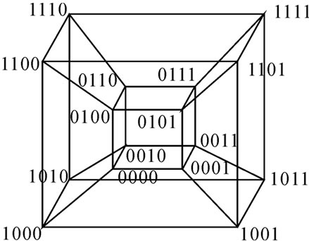
Figure 1. A 4-dimensional hypercube interconnection network.
finite field Fq, Notes that q is fairly large prime number and for any variables x and y, f(x,y)= f(y,x) is always held. Then the key server computes a share of f(x,y), denoted as f(i,y) for each node, where i is assumed to be a unique ID for any sensor node. Every node is pre-loaded with its own share before node-deployment phase. Thus for any two nodes i and j, node i can compute the common key f(i,j) by evaluating f(i,y) at point j, and vice visa.
To predistribute pairwise key with such a scheme as addressed above, node i's storage overhead includes two parts: One is (t+1)log q storage space for storing a tdegree polynomial f(i,y), the other is the storage space for its own ID information. [4] shows that this scheme has ability of t-collusion resistant. That is, if there exists no more than t compromised nodes in the network, the scheme can ensure the pairwise key is secure between any two normal nodes.
2.2.2. Polynomial Pool-based Key Predistribution
Pairwise key establishment in this scheme is processed in the following three phase: polynomial pool generation and key predistribution, direct key establishment, and path key establishment.
1) polynomial pool generation and key predistribution: This phase is mainly concerned with t-degree bivariate polynomial pool (F) generation over a finite field Fq. Then a subset Fi F is selected and the shares of all of the polynomials in this subset are assigned to the node i.
2) direct key establishment: Assume that node i and j wants to establish pairwise key, if they have a common share on a same polynomial, they can establish pairwise key by utilizing the polynomial-based scheme. This phase is performed as follows: node i may broadcast an encryption list,  ,
,  , v=1,2,…, |Fi|, where Kv is the share of the vth polynomial at point j. If node j can decrypts any one of these correctly, that means there exists a common share between the two nodes.
3) path key establishment: If there no pairwise key existent between node i and j, it’s necessary to find a key path defined in Definition3. Then the two nodes transmits secret information for pairwise key generation on this path.
2.2.3. Random Subset Assignment and Hypercube-Based Assignment
1) Random Subset Assignment: Different from polynomial scheme, the main idea of this assignment is to pick a random subset of polynomial pool, denoted as Fi F, and assign the share of this subset to node i.
2) Hypercube-based Assignment: Based on the concept of random subset, this assignment generates polynomial pool by utilizing hypercube model, and assign subsets to nodes according to node’s ID.
3. H2 (Hierarchical Hypercube) Model
Definition 5 (H2 diagram): Assume that there exist 2n nodes, the construction algorithm of n-dimension H2(n) is illustrated as follows:
1) Each  nodes are connected as a
  dimensional hypercube, in which nodes are coded from
  -
- , and such kind of node code is called Inner-Hypercube-Node-Code. As a result,
  different such kind of
  dimensional hypercubes can be formed, where
  represents the upper integer operation, and
  means the lower integer operation.
2) The obtained  different such kind of
  dimensional hypercubes are codes from
  -
- , and such kind of node code is called Outer-Hypercube-Node-Code. And then, the nodes in the
  different such kind of
  dimensional hypercubes with the same Inner-Hypercube-Node-Code are connected as a
  dimensional hypercube, so we can obtain
  different such kind of
  dimensional hypercubes.
3) The graph constructed through the above two steps is called a H2 graph. And it is obvious that each node in the H2 graph is coded as (r,h), where r ( ≤r≤
≤r≤ ) is the node’s Inner-Hypercube-Node-Code, and h (
 ≤h≤
≤h≤ ) is the node’s OuterHypercubeNode-Code.
Theorem 1: There exist 2n in H2(n) diagram.
Proof: The conclusion is naturally held as 2n=  *
* .
.
Theorem 2: The diameter of H2 (n) is n.
Proof: As the diameter of  dimension hypercube is
 , and it is naturally held for the case of
  dimension hypercube. Thus the diameter of H2(n) is
  +
+ =n according to definition5.
Theorem 3: The distance of any two nodes A(r1,h1) and B(r2,h2) in H2(n) is expressed as d (A,B)= dh(r1, r2)+dh(h1, h2)+1 where dh is Hamming distance.
Proof: Since the distance of any two nodes is the Hamming distance of their corresponding codes, it is held according to definition5.
4. Pairwise Key Establishment Scheme Based on H2 Model
As addressed above, polynomial-based and polynomoial-based schemes have some limitations. In this section we propose a new pairwise key establishment and predistribution scheme based on H2 model. The new algorithm is composed of three phases: polynomial pool generation and key predistribution, direct key establishment, and path key establishment.
4.1. Polynomial Pool Generation and Key Predistribution
Assume that there are N nodes in a wireless sensor network, where 2n-1< N  2n. A n-dimension H2(n) is then generated and we construct a polynomial pool with the following method:
1) The key setup server randomly generates n*2n bivariate t-degree polynomial pool over a finite fields Fq ,denoted as F={ (x,y),
  (x,y)| 0
 1,1
1,1 i
i
 , 0
, 0
 1,1
1,1 j
j
 }.
}.
2) The  bivariate polynomials, denoted as {
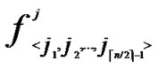 (x,y)| 0

 1}, where 1
 j
j
 , are assigned to the jth dimension of the
  th hypercube in H2(n).
3) The  bivariate polynomials, denoted as{
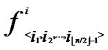 (x,y)| 0
 1} where1
  i
i
 , are assigned to the ith dimension of the
  th hypercube in H2(n).
4) For any nodes ( ,
, ) in H2(n), the polynomial shares, denoted as {
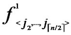 (x,y),
  (x,y),…,
  (x,y)}
  {
{ (x,y),
  (x,y),…,
  (x,y)}, are assigned and pre-loaded before deployment phase.
5) The server assigns a unique ID, denoted as ( ,
,  , to every node in sequence, where 0
 1, 0
1, 0

 1.
1.
4.2. Direct Key Establishment
If any two nodes A( ,
, ) and B(
 ,
, ) want to establish pairwise key, the node A can achieve the pairwise key with B by processing the following procedures:
Node A first computes the Hamming distance between B and itself, as d1=dh( ,
, ), d2=dh(
 ,
, ). If d1=1 or d2=1, the node can establish the pairwise with the peer according to the conclusion of the Theorem 4.
Theorem 4: For any two nodes A( ,
, ) and B(
 ,
, ), If the Hamming distance dh(
 ,
, )=1, or dh(
 ,
, ) =1, then there exists certainly pairwise key between A and B.
Proof: 1) dh( ,
, )=1: Assume that it=
 , where 1
 t
t
 -1. Since


 (
( ,
, ) =
) = (
( ,
, ). So, There exists a pairwise key
  (
( ,
, ) between A and B.
2) dh( ,
, )=1: Imitating the step 1), it is easy to prove that there exists a pairwise key between A and B.
4.3. Indirect Key Establishment
If dh( ,
, )>1 and dh (
 ,
, ) >1 then node A establish indirect pairwise key with B according to Theorem 5. In order to make it clear, we will provide a lemma before the illustration of Theorem 5.
Lemma1: For any two nodes A( ,
, ) and B(
 ,
, ), assume that dh=k, then there exists a k-distance path denoted as I0(=A), I1,…,Ik-1, Ik(=B), where dh (Ii,Ij)=1.
Proof: According to Theorem 3, dh can be expressed as dh( ,
, )+dh(
)+dh( ,
, )=k. Assume that dh(
 ,
, )=h, then dh(
 ,
, )=k-h. According to definition5, node C(
 ,
, ) and A are located in a
  -dimensional hypercube H, and node C and B are located in a
  -dimensional hypercube
 . According to the properties of hypercube [5,6], there exist a path described as I0(=A), I1,…, Ih-1, Ih(=C) in H, where dh(Ii, Ij)=1. Similarly, another path with the same property is existed in
 , denoted as Ih(=A), Ih+1, …, Ik-1, Ik(=B), where dh (Ii,Ij)=1.
Thus there exist a integrated path in H2 diagram from node A to B, described as I0(=A), I1,…,Ik-1, Ik(=B) where dh (Ii, Ij)=1.
Theorem 5: Assume that any two nodes can communicate directly in a wireless sensor networks, and there is no compromised node in the networks, then there exist a key path for any node A( ,
, ) and node B (
 ,
, ).
).
Proof: According to Lemma1, there exist a path for any two nodes where dh=k in H2 diagram. Thus the conclusion is held.
We propose the algorithm for indirect key establishment as follows. Assume the two nodes A( ,
, ) and node B(
 ,
, ) want to establish indirect pairwise key in the network, we propose the algorithm for indirect key establishment illustrated as follows.
Indirect_Key_Establishing_Algorithm(){
1) Node A computes a set L which records the dimensions in which node A and B have different sub-indexes. The set can be expressed as L={(d1,d2,…,dk),(g1,g2,…,gw)} where d1< d2< …< dk, g1< g2< …< gw.
2) Node A maintains a path set P with initial vale of P={A}.
3) Assume that U( ,
, ) =A; s=1.
4) Node A computes intermediate nodes expressed as V=( ,
, ). And P=P
 {V}.
{V}.
5) Assume that U =V.
6) If s< k, then s=s+1, and repeats the step 4, otherwise turns to step7).
7) Node A computes intermediate nodes V= ( ,
, ), and let P=P
 {V}.
{V}.
8) Let U =V.
9) If s< w, then s=s+1, and repeats step7); otherwise go on step10).
10) Let P=P {B}.
{B}.
}
According to Theorem 5, any node can compute a key path to it destination when there is no compromised node in the network. Once the path P is achieved, the two nodes can exchange secret information to generate pairwise key between themselves.
For example, the node A((001), (0101)) and the node B((100), (1100)) can establish pairwise key along the following key path: A((001), (0101)) ((101), (0101))
  ((100), (0101))
 ((100), (1101))
 B((100), (1100)).
According to the algorithm described above, the following conclusion is naturally held.
Theorem 6: Assume that any two nodes can communicate with each other directly, and there is no compromised node in a network. If the distance between the two nodes is k, then there exists a key path with distance of k. That is, the two nodes can establish pairwise key through k-1 intermediate nodes.
4.4. Dynamic Key Path Establishment
The Indirect_Key_Establishing_Algorithm() illustrated in Subsection 4.3 can only deal with the situation that there is no compromised node in the network. However, in case of some existent compromised nodes, the algorithm would fail to find fungible intermediate node to help establish pairwise key.
We further analyze the example addressed in Subsection 4.3. When the node ((101),(0101)) is compromised, the node A and B can utilize the following path to establish pairwise key: A((001), (0101)) ((000),(0101))
 ((100), (0101))
 ((100), (1101))
 B((100), (1100)).
When the node ((100),(1101)) is compromised, the two nodes can use the path: A((001), (0101))  ((101), (0101))
 ((100), (0101))
 ((100), (0100))
 B((100), (1100)).
In case that the nodes ((101),(0101)),((100),(1101)) are compromised, there still exists a key path denoted as A((001),(0101)) ((000),(0101))
 ((100),(0101))
 ((100),(0100))
 B((100),(1100)).
4.4.1. Relative Definitions of Local Weak Connectivity
Definition 6: The nodes A and B in a n-dimensional hypercube Hn are called neighbors, if that there exists only one different bit in their binary strings.
Definition 7: The node A in an m-dimensional hypercube/sub-hypercube Hm is m-disconnected, iif that all links between A and every faultless node in Hm are fault. The node A in an m-dimensional hypercube/subhypercube Hm is reachable, iif that A is faultless and not m-disconnected.
Definition 8 (k-dimensional local-weak-connectivity): A n-dimensional hypercube Hn is k-dimensional local-weak-connected, if all reachable nodes in each k-dimensional sub-hypercube Hk (k 1) of Hn forms a connected graph, and the number of reachable nodes in Hk is bigger than
 .
.
Definition 9 (general local-weak-connectivity): An ndimensional hypercube Hn is general local-weakconnected, if there exists a h-dimensional sub-hypercube Hh (h k), which is local-weak-connected and includes Hk, as for each k-dimensional sub-hypercube Hk (k
 1) of Hn.
Figure 2 presents a 3-dimensional hypercube H3 with two fault nodes and a 3-disconnected node. According to the above two kinds of local-weak-connectivity concepts, it is easy to prove that all reachable nodes in H3 is global connected.
4.4.2. Global Connectivity of Local-Weak-Connected Hypercube
An n-dimensional hypercube Hn has  nodes, in which each node can be represented by a binary string and has n different links. So Hn has n
  different links totally.
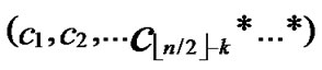
Definition 10: Any binary string
 …
… with given length n-k corresponds a k-dimensional sub-hypercube Hk with
  nodes, and the nodes in Hk can be represented by such binary strings as
 …
… *…*, where * can be 0 or 1.
From the construction algorithm of Hk, it is easy to know that all k-dimensional sub-hypercubes are isomor
Figure 2. A 3-dimensional hypercube H3 with fault nodes and links. In which, the black dots represent fault nodes, the white dots represent faultless nodes, the lines with tokens represent fault links, and the lines without tokens represent faultless links.
phic, and Hn includes all of the k-dimensional sub-hypercubes that is isomorphic with Hk. And it is easy to prove that Hn includes  -1 k-dimensional subhypercubes that is isomorphic with Hk and has no common nodes with Hk also.
Lemma 2: All of the reachable nodes in any two neighboring k-dimensional sub-hypercubes of the LocalWeak-Connected n-dimensional Hypercube Hn form a connected graph.
Proof: Let that Hk and  are two neighboring k-dimensional sub-hypercubes, according to definition 10, we can utilize binary strings
 …
… *…* to represent the nodes in Hk, where * can be 0 or 1. Since Hk and
  are neighboring, so there exists at least one common node between Hk and
 the nodes in
  can be represented as
 …
… *
* …
… *…*
*…* *…* and
 …
…

 …
… *…*
*…* *…*
*…* Hk.
Hk.
 …
…

 …
… *…*
*…* *…*
*…* Hk
Hk
 . Considering that the number of reachable nodes in
  is bigger than
 there exists at least one node A in those
  nodes represented by
 …
…

 …
… *… *
*… * *…* is reachable. Since A
 Hn
Hn Node A and all of the reachable nodes in
 form a connected graph. And in addition, since A

 Node A and all of the reachable nodes in
 form a connected graph also. So, all of the reachable nodes in Hk and
  form a connected graph.
Theorem 7: All of the reachable nodes in n-dimensional Hypercube Hn, which satisfies the conditions of k-dimensional local-weak-connectivity, form a connected graph.
Proof: From Theorem 2, it is easy to prove that the conclusion stands.
From Theorem 7, we can obtain the following deduces easily.
Deduce 1: If n-dimensional Hypercube Hn satisfies the conditions of k-dimensional local-weak-connectivity, then all of the reachable nodes in any h-dimensional sub-hypercube Hh(h k) form a connected graph.
Deduce 2: If n-dimensional Hypercube Hn satisfies the conditions of k-dimensional local-weak-connectivity, then there exists at least a pair of connected reachable nodes …
… 0
0 …
…
 …
… and
and …
… 1
1 …
…
 …
… between any pair of k-dimensional sub-hypercubes of
 …
… 0
0 …
… *…* and
 …
… 1
1 …
… *…*.
*…*.
Proof: From deduce 1, if n-dimensional Hypercube Hn satisfies the conditions of k-dimensional local-weak-connectivity All of the reachable nodes in any h-dimensional sub-hypercube Hh(h
 k) form a connected graph
  All of the reachable nodes in any (k+1)-dimensional sub-hypercube
 …
… *
* …
… *…* form a connected graph. And since the numbers of unreachable nodes in k-dimensional sub-hypercubes
 …
… 0
0 …
… *…* and
 …
… 1
1 …
… *…* are less than a half of the number of total nodes respectively. So, there exists reachable node
 …
… 0
0 …
…
 …
… in
in …
… 0
0 …
… *…*, and there exists reachable node
 …
… 1
1 …
…
 …
… in
in …
… 1
1 …
… *…* certainly. And in addition, those two nodes
 …
… 0
0 …
…
 …
… and
and …
… 1
1 …
…
 …
… is connected.
Theorem 8: All of the reachable nodes in n-dimensional Hypercube Hn, which satisfies the conditions of general local-weak-connectivity, form a connected graph.
Proof: Since n-dimensional Hypercube Hn is localweak-connected, and there exists no other sub-hypercubes that include itself in Hn. So, from definition 9, it is easy to know that Hn is n-dimensional local-weak-connected. And in addition, from definition 8, we can know that all of the reachable nodes in Hn form a connected graph.
Theorem 7 and Theorem 8 show that the hypercubes, that satisfy the conditions of the proposed two kinds of local-weak-connectivity, must be global connected.
4.4.3. K-Dimensional Local-Weak-Connectivity Based Dynamic Key Path Establishment Algorithm
KLWC-based Dynamic_Key_Path_Establishing_Algorithm(){
Input: Sensor network Hn with fault nodes and fault links (The links, whose length are bigger than the transmitting radius). And two reachable nodes A( ,
, ) and B(
 ,
, ) in Hn.
Output: A correct key path P from A to B in Hn.
1) Compute and determine the node T= ( ,
, ) in
) in ;
;
2) P=Dynamic_Key_Path_Establishment_1 (A,T);
3) P=P  Dynamic_Key_Path_Establishment_2 (T, B);
4) If P is a correct key path from A to B, then exit, otherwise turn to step 5);
5) Compute and determine the node T=( ,
, ) in
) in ;
;
6) P=Dynamic_Key_Path_Establishment_2 (A,T);
7) P=P  Dynamic_Key_Path_Establishment_1 (T, B);
8) If P is a correct key path from A to B, then exit, otherwise turn to step 9);
9) Report A, failure to establish a key path from A to B.
}
Algorithm Dynamic_Key_Path_Establishment_1(A,T):
1) Obtain the codes of nodes A and T: A (
( ,
, ), T
), T  (
( ,
, );
);
/* From definition 10, we can suppose that the k-dimensional sub-hypercube that includes T is ((
 …
… *…*),
*…*), ).*/
).*/
2) Initialize Path P: P A;
A;
3) Initialize temporary binary string C: C=( ,
, )
) A;
A;
4) FOR(j=1; j
 ; j++){
IF(

 ){
){
①According to lemma2 and deduce 1, a pair of connected reachable nodes C and D can be found through discovering in neighboring k-dimensional subhypercubes:
C=( ,
, )D=(
)D=( ,
, ), where
  =
= (t
(t [1, j]);
②Join the path from ( ,
, ) to node D into P;
③C D;
D;
}
}
/* After the above steps, a correct key path from node A( ,
, ) to the reachable node ((
 …
…
 …
… ),
), ) will be constructed. */
5) Join the path from node ((
 …
… ),
), ) to node T in the k-dimensional sub-hypercube ((
 …
… **),
**), ) into P. And then exit. So, a correct key path from node A to node T is discovered.
Algorithm Dynamic_Key_Path_Establishment_2(T, B):
1) Obtain the codes of nodes B and T: T  (
( ,
, ); B
); B  (
( ,
, );
);
/* From definition 10, we can suppose that the k-dimensional sub-hypercube that includes B is ( ,(
,(
 …
… *…*)).*/
2) Initialize Path P: P T;
T;
3) Initialize temporary binary string C: C=( ,
, )
)  T;
T;
4) FOR(l=1; l
 ; l++){
IF(

 ){
){
① According to lemma2 and deduce 1, a pair of connected reachable nodes C and D can be found through discovering in neighboring k-dimensional sub-hypercubes:
C=( ,
, );
);
D=( ,
, ), where
  =
= (t
(t  [1, l]).
②Join the path from ( ,
, ) to node D into P;
③ C D;
D;
}
}
/* After the above steps, a correct key path from node T( ,
, ) to the reachable node (
 , (
, (
 …
…
 …
… )) will be constructed. */
5) Join the path from node ( , (
, (
 …
…
 …
… )) to node B in the k-dimensional sub-hypercube (
 , (
, (
 …
… **)) into P. And then exit. So, a correct key path from node T to node B is discovered.
From the above description, we can know that the time complexity of algorithm Dynamic_Key_Path_ Establishment_1 is
 +
+ =
= , and the time complexity of algorithm Dynamic_Key_Path_Establishment_2 is
  +
+ =
= , so the total time complexity of the k-Dimensional LocalWeak-Connectivity based Dynamic Key Path Establishment Algorithm is
 .
.
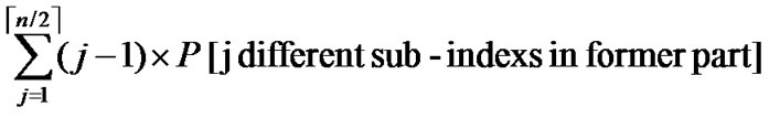
Considering the percentage of the fault nodes in sensor networks, when applying the k-Dimensional Local-Weak-Connectivity based Dynamic Key Path Establishment Algorithm actually, we can set k=1,2,3. Then the total time complexity of the k-Dimensional Local-Weak-Connectivity based Dynamic Key Path Establishment Algorithm will be  only. Figure 3 illustrates the relationship of dimension n and the scale of the sensor networks.
4.4.4. General Local-Weak-Connectivity Based Dynamic Key Path Establishment Algorithm
GLWC-based Dynamic_Key_Path_Establishing_Algorithm(){
Input: Sensor network Hn with fault nodes and fault links (The links, whose length are bigger than the transmitting radius). And two reachable nodes A( ,
, ) and B(
 ,
, ) in Hn.
Output: A correct key path P from A to B in Hn.
1) Compute and determine the node T=( ,
, ) in
) in ;
;
2)P=Dynamic_Key_Path_Establishment_3(A, T);
3)P=P  Dynamic_Key_Path_Establishment_4(T, B);
4)If P is a correct key path from A to B, then exit, otherwise turn to step 5);
5)Compute and determine the node T=( ,
, ) in
) in ;
;
6)P=Dynamic_Key_Path_Establishment_4(A, T);
7)P=P  Dynamic_Key_Path_Establishment_3(T, B);
8)If P is a correct key path from A to B, then exit, otherwise turn to step 9);
9)Report A, failure to establish a key path from A to B.
}
Algorithm Dynamic_Key_Path_Establishment_3(A, T):
1)Obtain the codes of nodes A and T: A (
( ,
, ), T
), T (
( ,
, );
);
/* From definition 10, we can suppose that the k-dimensional sub-hypercube that includes T is ((
 …
… *…*),
*…*), ).*/
).*/
2)Initialize Path P: P A;
A;
3)Initialize temporary binary string C: C=( ,
, )
) A;
A;
4)FOR(j=1; j n; j++){
IF(

 ){
){
FOR(k=1; k n-j; k++){
IF(According to Theorem 8, a pair of connected reachable nodes C and D can be found through discovering in neighboring k-dimensional sub-hypercubes:
C=(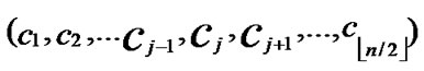 ,
, )D=(
)D=( ,
, ), where
  =
= (t
(t [1,j]);
①Join the path from
( ,
, ) to node (
 ,
, ) into P;
②C  (
( ,
,
 );
);
③Break;
}
}
IF(k >n-j){
WHILE(k n){
n){
IF(In the k-dimensional hypercube
( ,
, ), there exists no faultless key path from node C to node T) k++;
}
}
IF( k > n) exit. Then  is not general local-weak-connected, and we cannot find a correct key path from node A to T.
ELSE Join the path from C to T in the k-dimensional hypercube ( ,
, ) into P;
}
}
5) Exit. And a correct key path from A to T is discovered.
Algorithm Dynamic_Key_Path_Establishment_4(T, B):
1) Obtain the codes of nodes T and B: T  (
( ,
, ) and B
  (
( ,
, );
);
/* From definition 10, we can suppose that the k-dimensional sub-hypercube that includes B is ( ,(
,(
 …
… *…*)).*/
2) Initialize Path P: P T;
T;
3) Initialize temporary binary string C: C=( ,
, )
)  T;
T;
4) FOR(l=1; l n; l++){
IF(

 ){
){
FOR(k=1; k n-j; k++){
IF(According to Theorem 8, a pair of connected reachable nodes C and D can be found through discovering in neighboring k-dimensional sub-hypercubes:
C=( ,
, )D=(
)D=( ,
, )where
  =
= (t
(t [1,j]);
①Join the path from ( ,
,
 ) to node (
 ,
, ) into P;
②C  (
( ,
,
 );
);
③Break;
}
}
IF(k >n-j){
WHILE(k n){
n){
IF(In the k-dimensional hypercube ( ,
, ), there exists no faultless key path from node C to node B) k++;
}
}
IF(k > n) exit. Then  is not general local-weak-connected, and we cannot find a correct key path from node T to B.
ELSE Join the path from C to B in the k-dimensional hypercube ( ,
, ) into P;
}
}
5) Exit. And a correct key path from T to B is discovered.
From the above description, we can know that the time complexity of algorithm Dynamic_Key_Path_ Establishment_3 is  +
+ =
= , where
  is the smallest integer that satisfies the condition of k-dimensional local-weak-connectivity. And the time complexity of algorithm Dynamic_Key_Path_Establishment_4 is
  +
+ =
= , so the total time complexity of the general Local-WeakConnectivity based Dynamic Key Path Establishment Algorithm is
 .
.
Considering the percentage of the fault nodes in sensor networks, when applying the general LocalWeakConnectivity based Dynamic Key Path Establishment Algorithm actually, we can set k=1,2,3. Then the total time complexity of the General Local-WeakConnectivity based Dynamic Key Path Establishment Algorithm will be  only.
only.
5. Analysis
5.1. Feasibilities of the Algorithm
Theorem 9: In our algorithm, the possibility of direct key establishment for any two nodes can be expressed as PH2 (
( )/(N-1).
Proof: As the algorithm has assigned any node, denoted as ( ,
, ), shares of polynomials expressed as FA = {
 (j1,y),
  (j2,y),…,
  (
( ,y)}
,y)}  {
{  (i1,y),
  (i2,y),…,
  (
( ,y)}. It’s clear that there are
  nodes which can establish direct pairwise key with the node A. Thus PH2
 (
( )/(N-1) as the network scale is within the area 2n-1< N
  2n.
2n.
Suppose that a sensor network has N=10000 sensor nodes, then n=14. The possibility of direct key establish is about PH2 2.56% according to the conclusion drawn by Theorem 6. However, the possibility decreases to PH
 0.14% if the algorithm addressed in [3] is used.
Theroem10: Assume that the possibility of direct key establishment in H2-based scheme is defined as PH2, while the possibility in hypercube is denoted as PH, then PH2>>PH.
Proof: Suppose the number of a network is within the area of 2n-1< N  2n, and PH
 as addressed in [3]. Thus
  =
= =0.
=0.
5.2. Overhead AnalysisNode’s Storage Overhead
1) Any node is required to store t-degree bivariate polynomials whose number is n over the finite fields q, which occupies n(t+1)log q bits.
2) In order to keep the security of the Keys, for any bivariate polynomial f(x,y), node A is required to store the ID information of the compromised nodes that can establish direct key with A by using f(x,y). Since the degree of f(x,y) is t, then f(x,y) will be divulged when there are more than t nodes are compromised. So, for any bivariate polynomial f(x,y), node A needs only to store the ID information of n compromised nodes that can establish direct key with A by using f(x,y). In addition, since the node’s ID is a vector of n bits, and from Theorem 4, we can know that node A needs only to store one bit for each compromised node to determine the whole ID information of the compromised node. So, the total storage cost is nt bits.
3) Also the node’s own ID information occupies about n bits storage space, as it is expressed as ( ,
, ).
).
All of the storage overhead address above sum up to n(t+1)log q+nt+n= n(t+1)log 2q bits.
Theorem 11: The H2-based and the hypercube-based schemes have the same storage overhead.
Proof: According to the analysis on storage overhead addressed in Subsection 5.4 in [3], the result is certainly held.
Communication Overhead
In a sensor network, sending a unicast message between two arbitrary nodes may involve the overhead of establishing a route. In case of no compromised node existent in the network, any one node can communicate with the others directly. Assume that the overhead for a hop is defined as 1, then for two arbitrary nodes whose Hamming distance is L, the minimum communication overhead is L. We further inspect average communication overhead on H2-based path key establishment.
Suppose there are two nodes A( ,
, ) and B(
 ,
, ) In the formal part of node’s code, the probability of
  =
= , e
, e {1,…,
{1,…,  } is 1/2; Similarly, the probability of
  =
= , e
, e {1,…,
{1,…,  } is also 1/2 in the latter code part. Thus the probability for the two nodes to have i different sub-index in the formal part is expressed as P[i different sub-indexs in former part]=
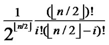 . In the latter part, we also have:
P[j different sub-indexs in later part]=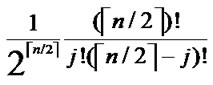 .
.
Thus the average communication overhead can be summarized as:
L= +
+ .
.
Theroem12: The average communication overhead in the H2-based scheme is less than that in the hypercube-based scheme.
Proof: According to the analysis on communication overhead addressed in Subsection 5.4 in [3], the result is certainly held.
Figure 5 shows that the comparison on communication overhead between the H2-based scheme and the hypercube-based scheme.
5.3. Security Analysis
Here we put focus on two types of attacks against H2-based scheme: 1) An adversary may compromise pairwise key between any two nodes or prevent them to establish a pairwise key. 2) The adversary may focus its power to attack against the whole network, for purpose of lowering the probability of pairwise key establishment, or in creasing communication cost.
5.3.1. Attacks against Pairwise Key between Two Nodes
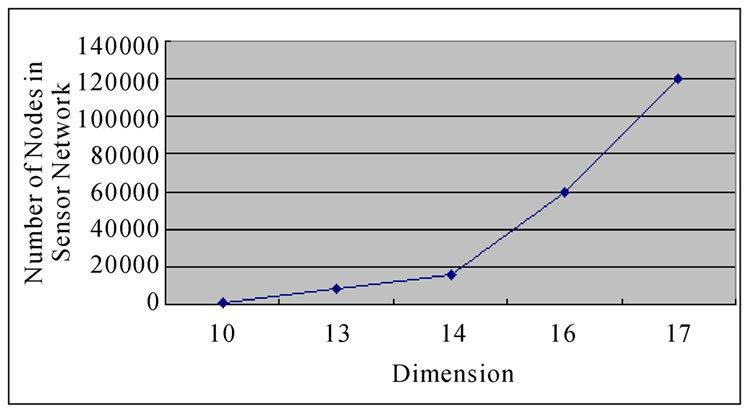
Figure 3. The relationship of dimension n and the scale of the sensor networks.
Figure 4. The comparison of probability to establish direct key between H2-based and Hypercube-based algorithms.
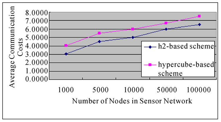
Figure 5. The comparison on average communication overhead between the H2-based and the Hypercube-based schemes.
1) Suppose an adversary launches an attack against two particular nodes, in order to filch their pairwise key. In case that those two nodes are not compromised:
① If the node u and v can establish direct pairwise key, the only means to compromise the key is to resolve the polynomial f(x,y), which is shared by the two nodes. As the degree of this polynomial is adversary t, the adversary is required to compromise at least t+1 compromised nodes with the same share of f(x,y).
② If the node u and v need to establish indirect pairwise key, the adversary is required to compromise an intermediate node, or filch the common share of the bivariate polynomial f(x,y) between the two nodes. However, even if the adversary succeeds to achieve the pairwirse key, the nodes u and v can also select alternatives to re-establish key path.
2) Suppose the adversary launch attacks to prevent pairwise key establishment against two particular nodes, denoted as u and v, which are assumed are not compromised. Then the adversary is required to compromise n bivariate polynomials of the node u or v. Notes that to those polynomials are t-degree, which means that if such attacks succeeded, at least n(t+1) nodes should have been compromised.
As addressed above and analysis presented in Subsection 5.5.1 in [3], if an adversary launches attacks against nodes, the security of the H2-based scheme if equivalent with that of the hypercube-based scheme. That is, we have the following theorem.
Theorem 13: The security of the H2-based scheme if equivalent with that of the hypercube-based scheme.
5.3.2. Attacks against the Whole Network
Suppose that an adversary has known the distribution state of polynomials for each node, he would launch attacks against the whole network systematically by compromising polynomials one by one. Assume that the adversary has compromised l bivariate polynomials, which means that at most  nodes have been pre-loaded one of those compromised polynomials. However, the rest of the regular nodes, denoted as N-
 do not contain compromised polynomial shares. That means N-
 nodes can still work properly. Notice that those regular nodes should avoid to use compromised shares to establish pairwise key.
Clearly, the number of nodes influenced by adversaries in the H2-based scheme is more than that in the hypercube-based scheme. However, on the condition that the adversary fails to compromise all of the polynomials, the effected nodes can select other regular nodes to establish pairwise key with others.
In addition, it has proved that the probability of direct key establishment in the H2-based scheme is much higher than that in the hypercube-based scheme. Thus in the process of direct key establishment among noncompromised nodes, the degree of the influence cause by adversaries on the H2-based scheme is less than that on the hypercube-based scheme. That means the the H2-based scheme has ability to secure communications among nodes effectively in sensor networks.
5.3.3. Security Performance
Based on the nice properties of fault tolerance in H2-baed scheme, a source node can re-establish pairwise key with the destination by selecting alternative key path.
As addressed in Subsection 4.1, the polynomial pool has n*2n bivariate t-degree polynomials, that is, |F|=n*2n; As every node contains n different polynomial shares, given a particular share of a bivariate polynomial f, the probability for each node to contain such a share is n/|F|. Assume that the number of nodes in a network is 2n-1< N  2n, and the number of supposed compromised node is
 , the probability for those compromised nodes to contain i shares of f is Pi=
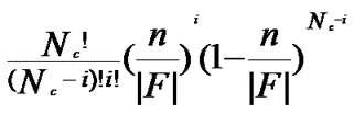
As the adversary needs to compromise at least t+1 nodes to filch f, the probability of being compromised for f is Pc=1- .
.
According to Theorem 6, the compromised probability of direct key establishment for any two non-compromised nodes is expressed as Plink= Pc PH2, in case that a particular polynomial f is compromised.
Figure 6 shows the fraction of compromised direct keys between non-comrpomised nodes as a function of the number of compromised keys for H2 and hypercube-based schemes where N=30000 and t=2.
Figure 6 shows that based on the assumption of same network scale and the proportion of compromised nodes, H2-based scheme provides higher probability than hypercube-based scheme for direct key establishment between any two non-compromised nodes. H2-based scheme would not fail to establish direct key until the proportion increases to 40%, while for Hypercube-based scheme, accepted proportion is about 30%.
We further inspect the probability of compromised indirect key. As addressed in Theorem 6, the probability of direct key establishment for any two nodes is PH2  (
( )/(N-1), the probability of indirect key establishment can be expressed as 1-PH. Thus the probability of compromised indirect key is estimated as (1-PH2) [1-(1-
 )
) (1-Pc)2].
Figure 7 shows that the probability of compromised indirect key between any two non-compromised nodes is a function of the fraction of compromised nodes where N=30000 and t =2.
Figure 7 shows that based on the same conditions of network scale and fraction of compromised nodes, H2-based scheme has better performance than hypercube-based scheme on indirect key establishment. The figure also shows that H2-based scheme would not fail to establish indirect key until the fraction of compromised nodes rises up to 60%. However, the fraction is only about 40% for Hypercube-based scheme.
Here we consider overall security performance of the two schemes. We define the probability of compromised pairwise key ( direct or indirect key) is Pkey=PH2 Pc+(1-PH2)[1-(1-
 )
)
 ].
].
Figure 8 shows that the probability of compromised pairwise key is a function of the fraction of compromised nodes where N=30000 and t=2 for the two schemes.
From Figure 8, we can know that the probability of the pairwise key between any two non-compromised nodes when the H2-based scheme is applied, is lower than that when the Hypercube-based scheme is applied, supposing that the scale and percentage of compromised nodes of the sensor networks are the same.
So, from the above description, it is obvious that the security performance of the H2-based scheme is better than that of Hypercube-based scheme.
The Probability of Pairwise Key Re-estab-lishment
A source node has to re-establish key path to the destination once some intermediate nodes have been compromised. According to the previous presented two kinds of dynamic key path establishing algorithms, it is easy to know that the algorithms can find a new alternative key path certainly, when k =1,2 or 3, as long as the distribution of the compromised nodes in the whole sensor network satisfy the conditions of 1,2 or 3- dimensional local-weak-connectivity. Next, lets analyze the probability of pairwise key reestablishment when the distrivution of the compromised node do not satisfy the conditions of 1,2 and 3-dimensional localweakconnectivities.
According to the pairwise key establishment scheme addressed above, each node in a network is able to communicate  nodes to establish direct pairwise key. Assume that the fraction of compromised nodes is p, then the number of non-compromised nodes among
  is (1-p)* (
 ). On the condition that a key path is available among those non-compromised nodes, it’s certainly possible for a source node and the destination to establish indirect pairwise key. So, when the distrivution of the compromised node do not satisfy the conditions of 1,2 and 3-dimensional local-weak
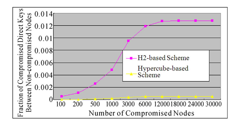
Figure 6. The relation between the fraction of compromised direct keys and the number of compromised nodes in H2- based scheme and Hypercube-based scheme.
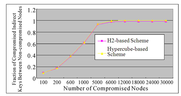
Figure 7. The comparison on the fraction of compromised indirect keys-number of compromised nodes relation between the H2-based scheme and the Hypercube-based scheme.
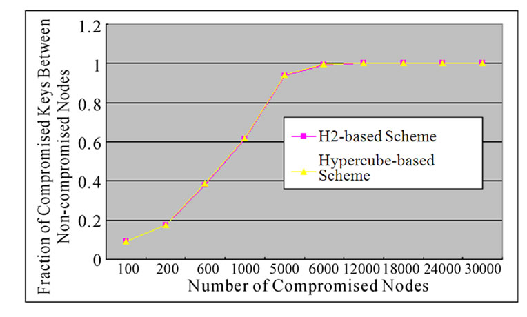
Figure 8. The comparison on the fraction of compromised keysnumber of compromised nodes relation between the H2-based scheme and the Hypercube-based scheme.
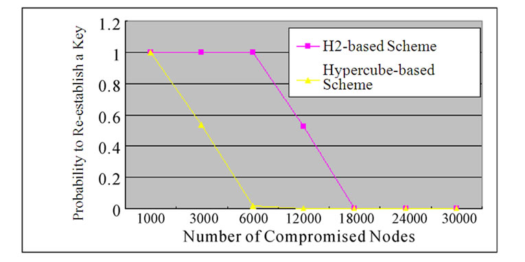
Figure 9. The relation between the probability of reestablished keys and the number of compromised nodes in the H2-based and Hypercube-based schemes.
connectivities, the probability of pairwise key re-establishment can be estimated as:
Pre=1-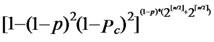
Assume that N=30000 and t=2, Figure 9 shows that the probability of pairwise key re-establishment is a function of number of compromised nodes in H2 and hypercube-based schemes. It also shows that the probability of pairwise key re-establishment in H2 scheme is higher than that in hypercube-based scheme for any two non-compromised nodes.
6. Conclusions
An H2-based key predistribution scheme is proposed. Compared with polynomial pool-based scheme, it can improve working performance on probability of direct key establishment without additional storage requirement.
Moreover, experimental figures show that our algorithm has lower communication cost and more secure than previous related works.
7. Acknowledgment
This work was supported in part by the China Scholarship Council (CSC) in form of a scholarship that funds the author, Lei Wang, studying at Lakehead University as a visiting researcher in Canada.
8. References
[1] L. Eeschnaure and V. D. Gligor, “A key-management scheme for distributed sensor networks,” in proceedings of the 9th ACM Conference on Computer and Communication Security, pp. 41-47, 2002.
[2] H. Chan, A. Oerrig, and D. Song, “Random key predistribution schemes for sensor networks,” in IEEE Syposium on Research in Security and Privacy, pp. 197-213, 2003.
[3] D. G. Liu, P. Ning, and R. F. Li, “Establishing pairwise keys in distributed sensor networks,” ACM Journal Name, Vol. 20, pp. 1-35, 2004.
[4] C. Blundo, A. Desantis, S. Kutten, et al., “Perfectly secure key distribution for dynamic conferences,” in Advances in Cryptology-CRYPTO’92, LNCS, 740, pp. 471-486, 1993.
[5] L. Wang and Y. P. Lin, “Maximum safety-path matrices based fault-tolerant routing for hypercube multi-computers,” Journal of Software, Vol. 15, No. 7, pp. 994-1004, 2004.
[6] L. Wang and Y. P. Lin, “A fault-tolerant routing strategy based on maximum safety-path vectors for hypercube multi-computers,” Journal of China Institute of Communications, Vol. 16, No. 4, pp. 130-137, 2004.