Wireless Sensor Network, 2011, 3, 263-274
doi:10.4236/wsn.2011.38027 Published Online August 2011 (http://www.SciRP.org/journal/wsn)
Multiple Targets Tracking Using Kinematics in Wireless
Sensor Networks
Akond Ashfaque Ur Rahman1, Atiqul Islam Mollah2, Mahmuda Naznin3
1Software Engineer-Dohatec New Media, Dhaka, Bangladesh
2Quantitative Software Developer-Stochastic Logic, Dhaka, Bangladesh
3Associate Professor-Department of C.S.E., BUET, Dhaka, Bangladesh
Received June 18, 2011; revised July 21, 2011; accepted July 31, 2011
Abstract
Target tracking is considered as one of the cardinal applications of a wireless sensor network. Tracking mul-
tiple targets is more challenging than tracking a single target in a wireless sensor network due to targets’
movement in different directions, targets’ speed variations and frequent connectivity failures of low powered
sensor nodes. If all the low-powered sensor nodes are kept active in tracking multiple targets coming from
different directions of the network, there is high probability of network failure due to wastage of power. It
would be more realistic if the tracking area can be reduced so that less number of sensor nodes will be active
and therefore, the network will consume less energy. Tracking area can be reduced by using the target’s ki-
nematics. There is almost no method to track multiple targets based on targets’ kinematics. In our paper, we
propose a distributed tracking method for tracking multiple targets considering targets’ kinematics. We si-
mulate our method by a sensor network simulator OMNeT++ and empirical results state that our proposed
methodology outperforms traditional tracking algorithms.
Keywords: Wireless Sensor Network, Multiple Targets, Tracking, Target Kinematics
1. Introduction
Now-a-days, from military applications (battlefield sur-
veillance and intelligence data acquisition), the use of
sensor networks has extended to many civilian, industrial
and environmental applications [1-2]. Among the diver-
sified applications of sensor networks, target detection is
one of the most important applications. In this context,
the primary tasks of a sensor network are targets ‘identi-
fication and classification, data acquisition, targets’ track-
ing or localizing and data transmission over multi-hop
networks [3]. Local information collected from sensor
nodes in a particular time frame is used to obtain the
global information regarding the location of the target.
But due to power constraint and frequent connectivity
failure of a sensor network, energy-efficient target track-
ing is a very challenging problem in the domain of sen-
sor networks. Not only we need to ensure the service
quality of the network, but also energy consumption
should also be minimized. A popular method to optimize
energy consumption in target tracking is the minimiza-
tion of tracking area; the region which is reachable by a
target from its current position with a certain speed. Pre-
vious works such as [4,5] employ this approach to track
targets efficiently. But they do not consider multiple
types of targets at a single time. In practical scenario, a
network has to detect multiple types of targets in a cer-
tain time frame. For example, in border surveillance,
sensor nodes have to detect multiple targets such as
wheeled vehicles or tracked vehicles such as tanks, or
biological entities (human, animals). A target tracking
methodology is desired to track all targets efficiently,
regardless of their types or numbers. In our paper, we
propose a novel, distributed, energy efficient multiple
targets tracking method which includes target classifica-
tion, data acquisition and transmission.
The core duties of detection, classification, tracking
and identity management, are devolved into three types
of sensor nodes, instead of confining into one. We use
the concept of target kinematics [6] in tracking multiple
targets to reduce the tracking area. It is not possible for a
target (tracked or wheeled) to traverse every portion of
its tracking area, because of its kinematics properties
such as steering angle and speed. If we can reduce the

264 A. A. U. RAHMAN ET AL.
tracking area, we can save energy consumption of the
whole network as fewer number of sensor nodes of the
tracking area are active. We have tried to reduce the
tracking area using heuristics based on overlapping crite-
ria. We have considered two ways of how these tracking
areas can overlap: one-one and one-two overlapping. In
the case of one-one overlapping, the tracking area of one
target simultaneously overlaps with one and only one
tracking area of one single target. In the case of one-two
overlapping, the tracking area of one target simultane-
ously overlaps with the tracking area of two targets. We
have provided heuristics and later explained those
through illustrative figures. We have simulated our algo-
rithm using a standard sensor network simulator OM-
NeT++ [7] to validate our method. Our proposed method
outperforms the traditional circular tracking area based
approaches in [4,5]. The remainder of this paper is or-
ganized as follows: section 2 describes the related re-
search work. In section 3, we give the preliminaries. In
section 4, we describe our tracking algorithm in details.
In section 5, we report the experimental results and em-
pirical analysis in form of tables and graphs. Finally,
section 6 gives the summary of our work with a direction
of future extension.
2. Related Work
In this section, we discuss some related research work.
Bar-Shalom et al. propose a centralized tracking method
where each sensor node transmits its sensing information
towards a processing node which acts as a central proc-
essor and fuses the report collected from all sensing
nodes [8]. Then, that processing node performs a long
distance transmission to the base station. But, this ap-
proach suffers from network latency and synchronization
problem, consumes huge amount of bandwidth and
eventually introduces a single point of failure. Besides,
the central node will be overloaded with computation.
In most of the sensor network applications, scalability
is an essential requirement also [3]. It can be achieved by
distributed tracking methods. In [4], Zhang et al. provide
a distributed, tree based algorithm which they call Dy-
namic Convoy Tree based Collaboration (DCTC), where
the sensor nodes track a single target. As a target moves
along its trajectory, the tree formed by the sensor nodes,
is continually reconfigured. Some nodes are added along
the predicted path and are pruned if they are not required.
Unfortunately, the construction of this convoy tree puts
an additional computational overhead over the sensor
nodes and it is almost impractical to implement.
In [9], Sikdar et al. use a linear prediction model to
track a single target. This prediction model performs
tracking based on the previous two observations. Even
though the model can be extended to predict higher order
predictions; these approaches require that all the sensor
nodes to be kept alive, which eventually minimizes the
lifetime of the network.
MCTA (Minimal Contour Tracking Algorithm), pro-
posed by Tian He et al. in their paper [5], is also another
centralized approach to track multiple targets. In their
method, each sensor node is assigned to track a particular
type of target which is a four-wheeled vehicle and sen-
sors nodes send tracking information to the base station.
Their computation is only applicable for tracking a cer-
tain type of targets, at a time. If there are other types of
targets such as a tank or any biological entity passing
through the network field, their algorithm will not be
able to track. Therefore, for this approach to work prop-
erly, all possible target entities and their kinematics
properties must be known.
3. System Architecture and Preliminaries
In this section, we describe our assumptions and defini-
tions which are relevant to our work. From the perspec-
tive of energy levels, we assume that the network con-
sists of two types of sensor nodes. A large portion con-
sists of typical low powered sensor nodes and a small
number of nodes with higher energy level are randomly
deployed. The high energetic nodes provide better con-
nectivity support [10]. According to responsibilities, we
classify the sensor nodes in to three categories namely,
Boundary Node (BN), Worker Node (WN) and Computa-
tional Node (CN). The sensor nodes that lie on the
boundary of the network field are called BN. We call the
high energetic nodes CN, as it will perform the necessary
calculations for detection, classification, tracking and
sleep-wake scheduling of the low powered sensor nodes.
Each CN is capable to relay target information to the
base station or to other CNs [10]. A WN senses and
transfers the target information. The whole tracking field
is mapped into Voronoi polygons with the CN as the Vo-
ronoi center [11-13]. We call each Voronoi polygon a
cell. Figure 1 describes a typical scenario of the network
field. Targets can enter into the network field from any
point on the boundary. There may be four types of tar-
gets: tracked vehicle, wheeled vehicle, biological entity
such as human being and animal.
The BNs are dedicated to target detection only. WNs
track targets and send information to the CN. At least
three active WNs are required to track a target according
to triangulation property [14]. WNs are responsible for
providing tracking information and their energy is pre-
served with the help of target kinematics. We prefer to
save BNs’ energy to prevent single point of failure [15]
in the sensor network. If all the BNs become out of power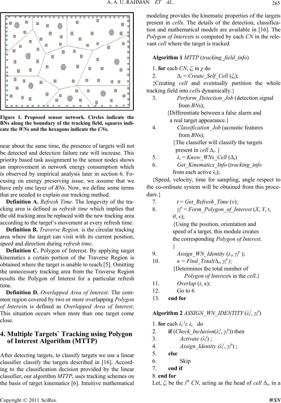

A. A. U. RAHMAN ET AL.
265
Figure 1. Proposed sensor network. Circles indicate the
BNs along the boundary of the tracking field, squares indi-
cate the WNs and the hexagons indicate the CNs.
near about the same time, the presence of targets will not
be detected and detection failure rate will increase. This
priority based task assignment to the sensor nodes shows
an improvement in network energy consumption which
is observed by empirical analysis later in section 6. Fo-
cusing on energy preserving issue, we assume that we
have only one layer of BNs. Now, we define some terms
that are needed to explain our tracking method.
Definition A. Refresh Time. The longevity of the tra-
cking area is defined as refresh time which implies that
the old tracking area be replaced with the new tracking area
according to the target’s movement at every refresh time.
Definition B. Traverse Region. is the circular tracking
area where the target can visit with its current position,
speed and direction during refresh time.
Definition C. Polygon of Interest. By applying target
kinematics a certain portion of the Traverse Region is
obtained where the target is unable to reach [5]. Omitting
the unnecessary tracking area from the Traverse Region
results the Polygon of Interest for a particular refresh
time.
Definition D. Overlapped Area of Interest. The com-
mon region covered by two or more overlapping Polygon
of Interests is defined as Overlapped Area of Interest.
This situation occurs when more than one target come
close.
4. Multiple Targets` Tracking using Polygon
of Interest Algorithm (MTTP)
After detecting targets, to classify targets we use a linear
classifier classify the targets described in [16]. Accord-
ing to the classification decision provided by the linear
classifier, our algorithm MTTP, uses tracking schemes on
the basis of target kinematics [6]. Intuitive mathematical
modeling provides the kinematic properties of the targets
present in cells. The details of the detection, classifica-
tion and mathematical models are available in [16]. The
Polygon of Interests is computed by each CN in the rele-
vant cell where the target is tracked.
Algorithm 1 MTTP (tracking_field_info)
1. for each CN, ζi in χ do
2. Δi = Create_Self_Cell (ζi);
{Creating cell and eventually partition the whole
tracking field into cells dynamically.}
3. Perform_Detection_Job (detection signal
from BNs);
{Differentiate between a false alarm and
a real target appearance.}
4. Classification_Job (acoustic features
from BNs);
{The classifier will classify the targets
present in cell Δi. }
5. λi = Know_WNs_Cell (Δi)
6. Get_Kin ematics_Info (tracking_info
from each active λi);
{Speed, velocity, time for sampling, angle respect to
the co-ordinate system will be obtained from this proce-
dure.}
7. t = Get_Refresh_Time (v);
8. γt
p = Form_Polygon_of_In terest (X, Y, t,
θ, v);
{Using the position, orientation and
speed of a target, this module creates
the corresponding Polygon of Interest.
}
9. Assign_ WN_Identity (λi, γt
p );
10. κ = Find_Total(Δi, γt
p );
{Determines the total number of
Polygon of Interests in the cell.}
11. Overlap (t, κ);
12. Go to 6
13. end for
Algorithm 2 ASSIGN_WN_IDENTITY (λi
j, γt p)
1. for each λi jε λi do
2. if (Check_Inclusion(λi
j, γt p)) then
3. Activa te (λi
j) ;
4. Assig n_Identity (λi
j, γt p) ;
5. else
6. Skip
7. end if
8. end for
Let, ζi be the ith CN, acting as the head of cell Δi, in a

266 A. A. U. RAHMAN ET AL.
tracking field χ, where, ζi ε ζ is the set of CNs in the
tracking field χ, and Δi ε Δ, is the set of cells formed in
the tracking field, χ. Here we consider the total network
which will track multiple targets as tracking field. We
also assume λi
j as the jth WN for ith cell Δi, in the tracking
field χ, where λi
j ε λi, the set of the WNs in ith cell Δi and
true for all i = 1. n in χ. Here, n is also the total number
of active cells in the tracking field χ, as the number of
active cells will be as same as the number of CNs in the
tracking field χ. Let us assume k to be the total number of
Polygon of Interests present in the ith cell, Δi, at time t.
Let, γt
p be the corresponding Polygon of Interest of target
p at any time t, in tracking field χ and μt
p, be the corre-
sponding area covered by the Polygon of Interest γt
p at
time t. The number of active WNs in a Polygon of Inter-
est γt
p is ηt p, for target p. We also call μt p,k to be the
Overlapped Area of Interest between μt
p and μt k, the cor-
responding area of Polygon of Interests, γt
p and γt k re-
spectively.
Algorithm 1 is the main module of MTTP. It provides
all the provisions to detect, classify and track multiple
targets. Algorithm 2 works as a sub-module to give the
identity of the WNs in a Polygon of Interest. Algorithm 3
is associated with overlap detection and calls the corre-
sponding modules. Algorithm 4, 5 and 6 are completely
responsible for overlap operations.
Algorithm 3 Overlap (t, κ)
1. for q = 1 to κ – 2
2. for w = q + 1 to κ – 1
3. for e = w + 1 to κ
4. if ((( Check_Overlap (γt
q , γt w)) &&
(Check_Overlap (γt
q , γt e)) &&
(Check_Overlap (γt
w , γt e))
= = true)
5. Get overlapped region of the three Poly
gon of Interests, γt
q , γt w , γt e; let it
be denoted as γt
q,w,e = γt r.
6. Get overlapped region of the two
Polygon of Interests, γt
q , γt w; let it
be denoted as γt
q,w
7. Get overlapped region of the two
Polygon of Interests, γt
q , γt e; let it
be denoted as γt
q,e
8. Get overlapped region of the two
Polygon of Interests, γt
w, γt e; let it
be denoted as γt
w,e
9. Simultaneous Overlapping of Three
Polygon of Interests (γt
q , γt w , γt e, γt r,
γt
q,w , γt q,e, γt w,e)
10. else
11. Take no action. Report that
simultaneous overlapping of
three Polygon of Interests have
not occurred.
12. end if
13. end for
14. end for
15. end for
16. for q = 1 to κ – 1
17. for w = q + 1 to κ
18. if ( Check_Overlap (γt
q, γt w))
19. Simultaneous Overlapping of Two
Polygon of Interests (γt
q, γt w)
20. else
Take no action. Report that
simultaneous overlapping of two
Polygon of Interests have not
occurred.
21. end if
22. end for
23. end for
For making WNs awake or asleep, we use the concept
of Polygon of Interest with the help of point in polygon
algorithm [13]. In case of overlapping, Overlapped
Polygon of Interests, are reconstructed on the basis of
mutual relativity, in size and properties of the Polygon of
Interests. We explore the internal details of our algorithm
in this section.
Algorithm 4 Simultaneous Overlapping of Three
Polygon of Interests (γt
a, γt b, γt c, γt d, γt e, γt f, γt g)
1. Get the area of the following contours γt
a , γt b, γt c and
γt
d. Let it be denoted as µt a, µt b, µt c and µt d respec-
tively.
2. Compute γt
a1, which will be the portion of γt a in-
cluded in γt
d.
3. Compute γt
b1, which will be the portion of γt b in-
cluded in γt
d.
4. Compute γt
c1, which will be the portion of γt c in-
cluded in γt
d.
5. Compute γt
e1, which will be the portion of γt e in-
cluded in γt
d.
6. Compute γt
f1, which will be the portion of γt f in-
cluded in γt
d.
7. Compute γt
g1, which will be the portion of γt g in-
cluded in γt
d.
8. Compute µt
a1, µt b1 and µt c1 from γt a1, γt b1 and γt c1 re-
spectively.
9. Get the updated area µ`t
a , µ`t b and µ`t c using µ`t a =
µt
a – µt a1, µ` t b = µt b – µt b1 and µ`t c = µt c – µt c1 respec-
tively and update γt
a , γt b , γt c as γ`t a , γ`t b and γ`t c re-
spectively.
10. Get the updated area µ`t
e, µ` t f and µ` t g using µ`t e =

A. A. U. RAHMAN ET AL.
267
µt
e – µt e1, µ` t f = µt f – µt f1 and µ`t g = µt g – µt g1 respec-
tively and update γt
e , γt f , γt g as γ`t e , γ`t f and γ`t g re-
spectively.
11. Calculate ηt
1, ηt 2 and ηt 3 from γ`t a , γ`t b and γ`t c re-
spectively.
12. If (ηt
1 => 3)
13. Individual Minimization (γ`t
a, γ`t e, γ`t f)
14. Else
15. Preserve γt
a. No minimization will take place.
Return γt
a
16. If (ηt
2 => 3)
17. Individual Minimization (γ`t
b, γ`t e, γ`t g)
18. Else
19. Preserve γt
b. No minimization will take place.
Return γt
b
20. If (ηt
3 => 3)
21. Individual Minimization (γ`t
c, γ`t f, γ`t g)
22. Else
23. Preserve γt
c. No minimization will take place.
Return γt
c
For simplicity, to describe the overlapping issue we
consider two Polygon of Interests of two targets at a cer-
tain time t. We check overlapping, by relatively detecting
the inclusion of one Polygon of Interest into another. The
WNs remain completely static during tracking. The
Polygon of Interests is reconstructed in such a way that
each of the Polygon of Interest possesses the sufficient
number of WNs to track the targets. Let two Polygon of
Interests be, γt
a and γt b where μt a and μt b, are respectively
their areas. The number of WNs in γt
a and γt b is respec-
tively denoted as, ηt
a and ηt b. We check the inclusion of
γt
b, which we call the Compared Polygon of Interest into
the Comparing Polygon of Interest, γt
a. If the inclusion is
true we consider the two Polygon of Interests to be over-
lapped. Then we calculate the area common between the
Polygon of Interests, γt
a, γt b and denote it as μt a,b. We then
adjust μt
b, which represents the area of Compared Poly-
gon of Interest γt
b, by subtracting μt a,b from it. ηt a, ηt b, ηt a,b
is also adjusted accordingly. We illustrate three cases
based on the value of ηt
b .
Algorithm 5 Individual Minimization (γt
1, γt 2, γt 3)
1. Compute γt
x as the area of γt 1 which is included in
the area of γt
2
2. Compute γt
y as the area of γt 1 which is included in
the area of γt
3
3. Compute µt
x and µt y from γt x and γt y respectively
4. Calculate γt
1 as γt 0 using µt 0 = µt 1 – µt x
5. Calculate γt
1 as γt 9 using µt 9 = µt 1 – µt y
6. Calculate ηt
9 and ηt 0.
7. If (ηt
9 => 3 || ηt 0 => 3)
8. Calculate ηt
Factor = Minimum (ηt 9, ηt 0)
9. If ηt
Factor => 3
10. Compute γt
Factor in correspondence to
ηt
Factor
11. Preserve γt
Factor
12. Else
13. Calculate ηt
Factor = Maximum (ηt 9, ηt 0)
14. Compute γt
Factor in correspondence to
ηt
Factor
15. Preserve γt
Factor
16. Return γt
Factor
17. Else
18. Preserve γt
1
19. Return γt
1
In the following illustration we study how Overlapped
Area of Interests effect the tracking decision policy while
tracking multiple targets. Larger Overlapped Area of
Interest between two Polygon of Interests results in
smaller number of WNs in that Polygon of Interest.
CASE 1. Here, we describe a certain situation that can
take place in the sensor network when two targets are
very close to each other. In this case, the corresponding
Polygon of Interests overlap each other by a large
amount. Figure 2 is the illustration of CASE 1. Here in
Figure 2(a), X and Y represent the Polygon of Interests
of two different targets, where X and Y are the Comparing
Polygon of Interest and Compared Polygon of Interest
respectively. According to our algorithm, size of Y is
reduced by the overlapped portion after detecting over-
lapping. Therefore, the number of WNs included in
Compared Polygon of Interest, but not in Overlapped
Area of Interest, is zero as indicated in Figure 2(b) (no
WNs in Y).
Algorithm 6 states that when the number of WNs in
the Compared Polygon of Interest, i.e., ηt
b is less than or
equal to one, the number of WNs in the Comparing
Polygon of Interest is divided by two and the similar
number of WNs is allocated to the both, Comparing
Polygon of Interest (X in Figure 2(c)) and Compared
Polygon of Interest (X in Figure 2(c)).
Figure 2. Illustration of Case 1.

268 A. A. U. RAHMAN ET AL.
Algorithm 6 Simultaneous Overlapping of Two Poly-
gon of Interests (γt
q , γt l)
1. Get the overlapped area µt
q,l from µt q and µt l.
2. Update µt
l using µt l = µt l – µt q,l and adjust ηt l, accord-
ingly.
3. if ηt
l <= 1 then
4. η`t
q = Floor (ηt q / 2)
5. end if
6. if ηt
l == 2 then
7. η`t
q = Floor (ηt q / 3)
8. end if
9. Update γt
q such that ηt q = ηt q – η`t q
10. Update γt
l such that ηt l = ηt l + η`t l
CASE 2. Here, the margin of overlap among two tar-
gets is not as large in CASE 1. In Figure 3(a), X and Y,
represent the Polygon of Interest of two targets. As they
come close to each other, their respective Polygon of
Interests overlap. Necessary reduction is done from the
two Polygon of Interests and the number of WNs is cal-
culated. According to Figure 3(b), the number of WNs in
Compared Polygon of Interest (Y) but not in Overlapped
Area of Interest, is two. Algorithm 6 states when ηt
b, the
number of WNs in the present Compared Polygon of In-
terest is equal to two, the number of active WNs in the
Comparing Polygon of Interest γt
a, is divided by three
and the floor of the quotient is taken. We then add this
number of WNs to ηt
b. Subtraction from ηt a is done by the
same amount. The reallocation of WNs sets up the two
Polygon of Interests track their corresponding targets.
CASE 3. CASE 3 is also very simple. As the overlap
between the two Polygon of Interests are low, no sig-
nificant change occurs in the two Polygon of Interests as
stated in Figure 4. When the number of active WNs in
the Polygon of Interest ηt
b is equal to or greater than
three we consider it sufficient to track target with proper
id management. The value of ηt
a and ηt b is kept un-
changed.
CASE 4. We use Figures 5, 6 and 7 to explore the
mechanisms of our proposed methodology to describe a
scenario where three Polygon of Interests are overlapping.
There are three Polygon of Interests X, Y and Z according
to Figure 5(a). As Figure 5(b) states, there are three
Polygon of Interests namely; X, Y and Z are overlapped
with each other. As the condition (according to Algo-
rithm 3, line 4) to check overlap is fulfilled, according to
our algorithm (according to Algorithm 3, line 5) first of
all we need to get the common area of these three Poly-
gon of Interests.
Let this Polygon of Interest be named as D. We will
also calculate the Overlapped Area of Interest, A be-
tween X and Y; Overlapped Area of Interest, B between
X and Z; Overlapped Area of Interest, C between Y and
Z.
Figure 3. Illustration of Case 2.
Figure 4. Illustration of Case 3.
Figure 5. Illustration of CASE 4.
Now for each Polygon of Interest X, Y and Z the algo-
rithm Simultaneous Overlapping of Three Polygon of
Interests is called. First of all the area of X, Y, Z and D
will be calculated; let them be named respectively as
Area(X), Area(Y), Area(Z) and Area(D) (according to
Algorithm 4, line 1). Now we have to find that portion of
the Polygon of Interest X which is included in D. Let it
be named as X1. The same procedure is also applied to Y
and Z and the corresponding area is named as Y1 and Z1
respectively (according to Algorithm 4, line 2, 3, 4). We
know compute X`, Y` and Z` as X`= X – X1 (shown in
Figure 6(a)), Y`= Y – Y1 (shown in Figure 6(b)) and Z`=
Z – Z1 (shown in Figure 6(c)). X`, Y` and Z` is shown in
Figure 6(d) respectively.

A. A. U. RAHMAN ET AL.
269
5). We illustrate the calculation of X0 in Now we will calculate the Overlapped Area of Interest
between the Polygon of Interests X and Y, X and Z and Y
and Z and name them respectively as A, B and C. Now
we have to find that portion of A which is included in D;
we name it as D1. In the same manner we calculate D2
for B and D3 for C. We will then calculate A`, B` and C`
using A` = A – D1, B` = B – D2 and C`= C – D3 (accord-
ing to Algorithm 4, line 9). Result of these calculations
are shown in Figure 6(e) and it is evident from the figure
that then number of WNs in the Polygon of Interests A`,
B` and C` is one for each of the Polygon of Interests.
Figure 7(a1) and the calculation of X9 in
Figure 7(a2). We calculate the number of
WNs of X0 and X9 and denote them
respectively as n(X0) and n(X9). It is
evident that n(X0) = 3 and n(X9) = 3. We now
need to find the Polygon of Interest
XFactor, whose number of WNs included in
the Polygon of Interest is denoted as
n(XFacto r) and which will be the final result of
the algorithm Individual Minimization.
According to the figure Minimum (n(X0), We will now calculate the number of WNs in X`, Y`
and Z` and we denote them as n(X`), n(Y`) and n (Z` )
respectively (according to Algorithm 4, line 12). Ac-
cording to Figure 5(f), 5(g) and 5(h), n(X`) = 3, n(Y`) =
5 and n (Z`) = 4. As the numbers of WNs in each of the
minimized Polygon of Interests are greater than or equal
to 3, according to our algorithm the condition to call al-
gorithm Individual Minimization is fulfilled.
n(X9)) = 3. So, n(XFactor) = 3 (according
to Algorithm 5, line 8). As n(XFactor) fulfills
the condition so Polygon of Interest XFactor
as shown in Figure 7(a3) will be computed,
preserved and will be
returned (according to Algorithm 5, line 10).
The algorithm Individual Minimization will be called
(according to Algorithm 4, line 13) with the following
parameters: Polygon of Interest X`, A` and B`.
Calling algorithm Individual Minimization (Algorithm
5) with the following parameters, Polygon of Interest Y`,
A` and C`:
The algorithm Individual Minimization will be called
(according to Algorithm 4, line 17) with the following
parameters: Polygon of Interest Y`, A` and C`.
First of all, we will calculate the portion of
Y` which is included in A`; we name this
area as A2`. Then we calculate the portion
The algorithm Individual Minimization will be called
(according to Algorithm 4, line 21) with the following
parameters: Polygon of Interest Z`, B` and C`.
of Y` which is included in C` and name this
area as C2`. We update Y1 as Y1 = Y` – A2`
and Y2 as Y2 = Y` – C2` which is shown in
Figure 7(b1) and 7(b2). We calculate the Calling algorithm Individual Minimization (Algorithm
5) with the following parameters, Polygon of Interest X` ,
A` and B`:
number of WNs of Y1 and Y2 and denote
them respectively as n(Y1) and n(Y2). We
now need to find the Polygon of Interest First of all, we will calculate the portion of
X` which is included in A` (according to YFa ctor, whose number of WNs included in
the Polygon of Interest is denoted as Algorithm 5, line 1); we name this area as
A1`. Then we calculate the portion of X` n(YFactor) and which will be the final result
which is included in B` (according to of the algorithm Individual Minimization.
According to the figure Minimum (n (Y1), n Algorithm 5, line 2) and name this area as
B1`. We will create two Polygon of Interests (Y2)) = 4. So, n(YFactor) = 4. As n(YFacto r)
fulfills the condition so Polygon of Interest, X0 and X9 using X0 = X` – A1`
YFactor will be computed, preserved and (according to Algorithm 5, line 4) and
X9 = X` – B1`(according to Algorithm 5, line will be returned.
Figure 6. Illustration of CASE 4(Contd).

270 A. A. U. RAHMAN ET AL.
Figure 7. Illustration of CASE 4 (Contd.).
Calling algorithm Individual Minimization (Algorithm
5) with the following parameters, Polygon of Interest Z`,
B` and C`:
First of all, we will calculate the portion of
Z` which is included in B` ; we name this
area as B3`. Then we calculate the portion of
Z` which is included in C`and name this area
as C3`. We update Z1 as Z1 = Z` – B3` and
Z2 as Z2 = Z` – C3` which is shown in Figure
7( c1) and 7(c2). We calculate the number of
WNs of Z1 and Z2 and denote them
respectively as n(Z1) and n(Z2). We now
need to find the Polygon of Interest ZFactor,
whose number of WNs included in the
Polygon of Interest is denoted as n(ZFactor)
and which will be the final result of the
algorithm Individual Minimization.
As n(Z1) = 3 and n(Z2) = 3, according to the
figure Minimum (n(Z1), n(Z2)) = 3. So,
n(XFactor) = 3 (according to
Algorithm 5, line 8). As n(XFactor) fulfills
the condition (according to Algorithm 5, line
9) so Polygon of Interest XFactor
as shown in Figure 7(a3) will be computed
(according to Algorithm 5, line 10),
preserved (according to
Algorithm 5, line 11) and will be returned
(according to Algorithm 5, line 16).
The algorithm Simultaneous Overlapping of Three
Polygon of Interests can be reduced to describe the
mechanisms when one Polygon of Interest overlaps with
another Polygon of Interest, at a certain time. We call it
the Simultaneous Overlapping of Three Polygon of In-
terests Reduced to Two algorithm denoted by Algorithm
7. We assume it will need at least three WNs in one sin-
gle Polygon of Interest to track one single target.
Algorithm 7: Simultaneous Overlapping of Three
Polygon of Interests Reduced to Two (γt
a , γt b)
1. Get the area of the Polygon of Interests γt
a and γt b.
Let it be denoted as µt
a and µt b respectively.
2. Compute the overlapped area between µt
a and µt b
and let it be denoted as µt
c.
3. Compute γt
a1, which will be the portion of γt a in-
cluded in γt
c.
4. Compute γt
b1, which will be the portion of γt b in-
cluded in γt
c.
5. Compute µt
a1 and µt b1 from γt a1 and γt b1 respectively.
6. Get the updated area µ`t
a and µ`t b using µ`t a = µt a –
µt
a1 and µ`t b = µt b – µt b1 respectively and update γt a
and γt
b as γ`t a and γ`t b respectively.
7. Calculate η1 and η2 from γ`t
a and γ`t b respectively.
8. If (η1 => 3 )
9. Preserve minimization. Return γ`t
a .
10. Else
11. Preserve γt
a. No minimization will take
place. Return γt
a
12. If (η2 => 3 )
13. Preserve minimization. Return γ`t
b .
14. Else
15. Preserve γt
b. No minimization will take
place. Return γt
b.
We describe some case studies below to further illus-
trate the algorithm.
CASE 5. Here, we describe a certain situation that can
take place in the sensor network when two targets are
close to each other. In this case, the corresponding Poly-
gon of Interests overlap each other by a significant
amount. Figure 8 is the illustration of CASE 5. Here in
Figure 8(a), X and Y represent the Polygon of Interests
of two different targets. In Figure 8(b) the two Polygon
of Interests overlap. According to Algorithm 7, the
Overlapped Area of Interest of the two Polygon of Inter-
ests, X and Y will be calculated. Let it be named as Z.
Then the area of X and Y included in Z will be calculated
(Algorithm 7, line 5); let them be denoted as X1 and Y1

A. A. U. RAHMAN ET AL.
271
respectively. We will now calculate X` and Y` using X` = X
– X1 and Y` = Y – Y1 respectively (algorithm 7, line 6). The
calculations to find X` and Y` is represented in Figure 8(c)
and 8(d) respectively. Now we calculate the number of
WNs in X` and Y` and denote them as n(X`) and n(Y`). Ac-
cording to Figure 8(e), n(X`) = 3 and Figure 8(f), n(Y`) =
5.
Thus minimization will be preserved according to our
algorithm (line 9 and line 13). Polygon of Interests X` and
Y` is the final outcome of this study.
CASE 6. In this case, the corresponding Polygon of In-
terests overlaps each other by a small amount. Figure 9 is
the illustration of CASE 6. Here in Figure 9(a), X and Y
represent the Polygon of Interests of two different targets.
Figure 9(b) represents the overlap between the two Poly-
gon of Interests. According to our algorithm, first the
Overlapped Area of Interest of the two Polygon of Interests
namely, X and Y will be calculated. Let it be named as Z.
Then the area of X and Y included in Z will be calculated;
let them be denoted as X1 and Y1 respectively. We will
now calculate X` and Y` using X` = X – X1 and Y` = Y – Y1
respectively. Now we calculate the number of WNs in X`
and Y` and denote them as n(X`) and n(Y`). According to
Figure 9(c), n(X`) = 3 (Algorithm 7, line 7) and n(Y`) =
2.The minimization for Polygon of Interest X will be
preserved but minimization for Polygon of Interest Y will
not be preserved according to our algorithm 7 (line 15).
We will restore Polygon of Interest Y by adding Y = Y` +
Y1. The outcome of this case study are the Polygon of
Interests are X` and Y` as indicated in Figure 9(e) and 9(f)
respectively.
CASE 7. Figure 10 is the illustration of CASE 7. Here
in Figure 10(a), X and Y represent the Polygon of Inter-
ests of two different targets. In this case, the correspond-
ing Polygon of Interests overlaps each other by a small
amount as indicated in Figure 10(b). According to our
algorithm, first the Overlapped Area of Interest of the
two Polygon of Interests, X and Y will be calculated. Let
it be named as Z. Then the area of X and Y included in Z
will be calculated; let them be denoted as X1 and Y1 re-
spectively. We will now calculate X` and Y` using X` = X
– X1 and Y` = Y – Y1 respectively. Now we calculate the
number of WNs in X` and Y` and denote them as n(X`)
and n(Y`). According to Figure 10, n(X`) = 5 and n(Y`) =
5 and so the minimization will be preserved according to
our algorithm.
Figure 8. Illustration of CASE 5.
Figure 9. Illustration of CASE 6.

272 A. A. U. RAHMAN ET AL.
Figure 10. Illustration of CASE 7.
The minimizations for both the Polygon of Interests X
and Y have not occurred in terms of number of WNs as
the Overlapped Area of Interest Z did not contain any
WNs and hence the number of WNs in both the Polygon
of Interests remains unchanged.
5. Evaluation and Comparison
We simulate using a widely used sensor network simu-
lator OMNeT++ for validating our method. We keep the
settings (Table 1) same for all the simulation runs. We
set a realistic range for target speed to be 5 – 12 ms–1 (18
– 42 km per hour). For wheeled vehicles, the steering
angle is 20˚ in most of the cases [17]. A greater steering
angle at such speed is not realistic, and if it is considered,
the vehicle is expected to loop within a circular path well
inside the Polygon of Interest. The size of the Polygon of
Interest is dependent on the refresh time. Appropriate
algorithms [17] are used to determine an optimal refresh
time. To observe the performance of our tracking algo-
rithm, we simulate using two/three targets moving across
the sensor network at the same time, in all the simulation
runs. In our first experiment, we implement such a
tracking methodology where circular tracking area is
used.
We call it ‘Centralized Scheme’. We name our second
experiment as ‘Centralized Scheme with Target Kine-
matics’. In this experiment we implement MCTA [5]. In
the final experiment, we implement our tracking algo-
rithm, MTTP. In accordance to MTTP, we partition the
whole tracking field into cells, giving each CN authority
over the WNs in the relevant cell. Figure 11, 12 and 13
respectively; show the amount of energy consumed by
the CNs, WNs and the total network. Clearly, the first
approach that used circular tracking area consumes more
energy at each phase of the simulation. In Table 2, the
comparison among three methods is given. We find that
our method MTTP outperforms the circular tracking area
based algorithms as it prunes out the tracking area ap-
proximately by 50% while preserving up to 60% of total
energy.
Table 1. Simulation Settings.
Parameter Value
General Settings
Network Dimension 1000 × 1000 meter
Number of WNs 500
Number of CNs 1 to 10
Number of BNs 40
Deployment of nodes Uniform Random
Link types
1. BN to CN unidirectional, short range
2. WN to CN unidirectional, short range
3. CN to CN unidirectional, long range
Event Settings
Simulation type Discrete-event driven
Target intrusion point User defined
Inter-arrival time for targetsStatic
Target Mobility Type Brownian motion
Simulation Time 2500 STU
Energy Model
Initial Energy in WNs 100 J
Initial Energy in BNs 100 J
Initial Energy in CNs 2000 J
Power dissipation in radio
transmission 10–4 W/m2
WN energy dissipation rate Active Mode: 24 mW
Idle Mode: 45 μW
CN energy dissipation rate Active Mode: 24 mW
Idle Mode: 45 μW
Figure 11. Comparison of energy consumption at CNs.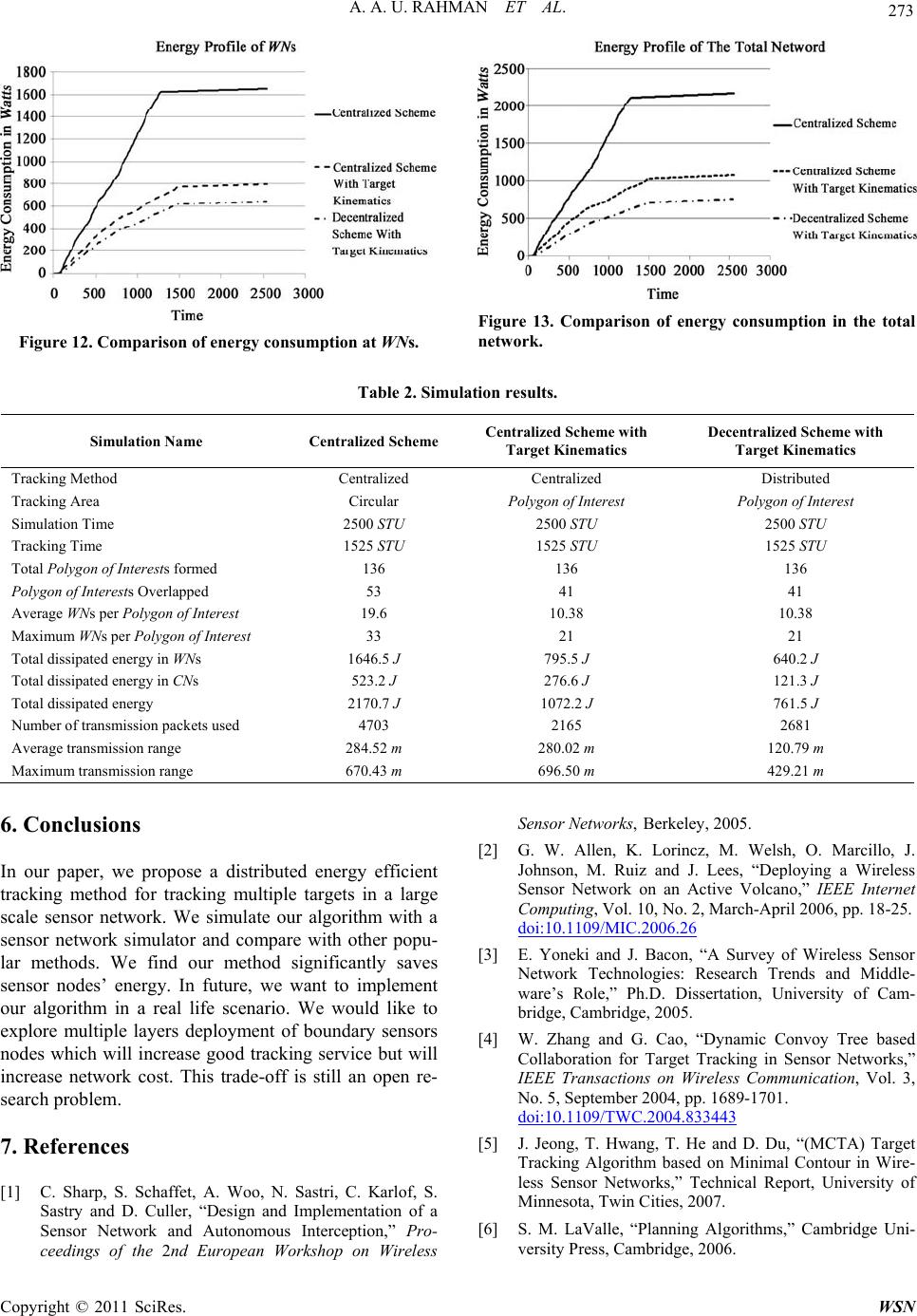

A. A. U. RAHMAN ET AL.
273
Figure 12. Comparison of energy consumption at WNs.
Figure 13. Comparison of energy consumption in the total
network.
Table 2. Simulation results.
Simulation Name Centralized Scheme Centralized Scheme with
Target Kinematics Decentralized Scheme with Target Kinematics
Tracking Method Centralized Centralized Distributed
Tracking Area Circular Polygon of Interest Polygon of Interest
Simulation Time 2500 STU 2500 STU 2500 STU
Tracking Time 1525 STU 1525 STU 1525 STU
Total Polygon of Interests formed 136 136 136
Polygon of Interests Overlapped 53 41 41
Average WNs per Polygon of Interest 19.6 10.38 10.38
Maximum WNs per Polygon of Interest 33 21 21
Total dissipated energy in WNs 1646.5 J 795.5 J 640.2 J
Total dissipated energy in CNs 523.2 J 276.6 J 121.3 J
Total dissipated energy 2170.7 J 1072.2 J 761.5 J
Number of transmission packets used 4703 2165 2681
Average transmission range 284.52 m 280.02 m 120.79 m
Maximum transmission range 670.43 m 696.50 m 429.21 m
6. Conclusions
In our paper, we propose a distributed energy efficient
tracking method for tracking multiple targets in a large
scale sensor network. We simulate our algorithm with a
sensor network simulator and compare with other popu-
lar methods. We find our method significantly saves
sensor nodes’ energy. In future, we want to implement
our algorithm in a real life scenario. We would like to
explore multiple layers deployment of boundary sensors
nodes which will increase good tracking service but will
increase network cost. This trade-off is still an open re-
search problem.
7. References
[1] C. Sharp, S. Schaffet, A. Woo, N. Sastri, C. Karlof, S.
Sastry and D. Culler, “Design and Implementation of a
Sensor Network and Autonomous Interception,” Pro-
ceedings of the 2nd European Workshop on Wireless
Sensor Networks, Berkeley, 2005.
[2] G. W. Allen, K. Lorincz, M. Welsh, O. Marcillo, J.
Johnson, M. Ruiz and J. Lees, “Deploying a Wireless
Sensor Network on an Active Volcano,” IEEE Internet
Computing, Vol. 10, No. 2, March-April 2006, pp. 18-25.
doi:10.1109/MIC.2006.26
[3] E. Yoneki and J. Bacon, “A Survey of Wireless Sensor
Network Technologies: Research Trends and Middle-
ware’s Role,” Ph.D. Dissertation, University of Cam-
bridge, Cambridge, 2005.
[4] W. Zhang and G. Cao, “Dynamic Convoy Tree based
Collaboration for Target Tracking in Sensor Networks,”
IEEE Transactions on Wireless Communication, Vol. 3,
No. 5, September 2004, pp. 1689-1701.
doi:10.1109/TWC.2004.833443
[5] J. Jeong, T. Hwang, T. He and D. Du, “(MCTA) Target
Tracking Algorithm based on Minimal Contour in Wire-
less Sensor Networks,” Technical Report, University of
Minnesota, Twin Cities, 2007.
[6] S. M. LaValle, “Planning Algorithms,” Cambridge Uni-
versity Press, Cambridge, 2006.

274 A. A. U. RAHMAN ET AL.
[7] OMNeT++ Community Site. http://www.omnetpp.org
[8] Y. Bar-Shalom and T. E. Fortmann, “Tracking and Data
Association,” Academic Press Professional, San Diego,
1987.
[9] H. Yang and B. Sikdar, “A Protocol for Tracking Mobile
Targets Using Sensor Networks,” Proceedings of the
IEEE Workshop on Sensor Network Protocols and Ap-
plications, Vol. 7, 2003, pp. 71-81.
doi:10.1109/SNPA.2003.1203358
[10] Tinynode. http://www.tinynode.com
[11] W. AlSalih, K. Islam, Y. N. Rodriguez and H. Xiao,
“Distributed Voronoi Diagram Computation in Wireless
Sensor Networks,” Proceedings of the 20th ACM Sympo-
sium on Parallelism in Algorithms and Architectures
(SPAA), 2008, p. 364. doi:10.1145/1378533.1378597
[12] X. Du and F. Lin, “Maintaining Differentaited Coverage
in Heterogenous Sensor Networks,” EURASIP Journal on
Wireless Communication and Networking, Vol. 2005, No.
54, August 2002, pp. 459-461.
doi:10.1155/WCN.2005.565
[13] Bob Stein, “A Point About Polygons,” Linux Journal,
March 1997.
[14] J. A. Stankovic, T. Abdelzaher, and T. He, “Lightweight
Detection and Classification for Wireless Sensor Net-
works in Realistic Environments,” Proceedings of the 3rd
ACM Conference on Embedded Networked Sensor Sys-
tems, San Diego, November 02 - 04 2005, pp. 205-217.
doi:10.1145/1098918.1098941
[15] R. R. Brooks, P. Ramanathan and A. M. Sayeed, “Dis-
tributed Target Classification and Tracking in Sensor
Networks,” Proceedings of the IEEE, Vol. 31, No. 8,
2003, pp. 1163-1171. doi:10.1109/JPROC.2003.814923
[16] A. U. R. Akond, M. A. I. Mollah and M. Naznin, “Multi-
ple Targets Tracking in Wireless Sensor Networks using
Target Kinematics,” Undergraduate Thesis, Bangladesh
University of Engineering and Technology, Dhaka, 2009.
[17] D. R. Kincaid and W. W. Cheney, “Numerical Analysis
the Mathematics of Scientific Computing,” American
Mathematical Society, Rhode Island, 2002.
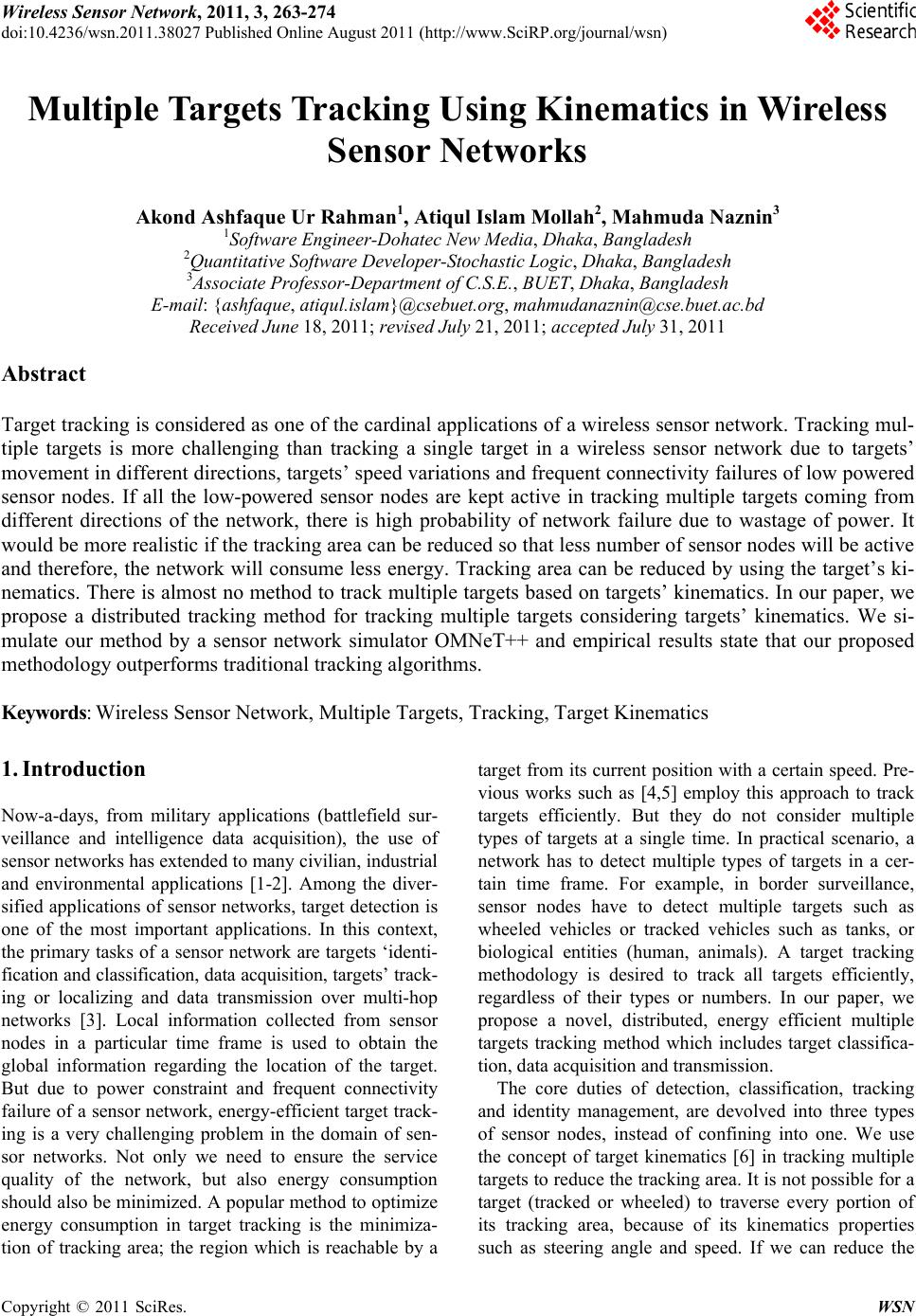