International Journal of Geosciences, 2011, 2, 231-239
doi:10.4236/ijg.2011.23025 Published Online August 2011 (http://www.SciRP.org/journal/ijg)
Three-Dimensional Representation of Geochemical Data
from a Multidimensional Compositional Space
Pietro Armienti, Placido Longo
1Dipartimento di Scie nze del l a Terra , Università di Pisa, Pisa, Italy
2Dipartimento di Matematica Applicata, Università di Pisa, Pisa, Italy
Received January 2, 2011; revised May 3, 2011; accepted July 8, 2011
Abstract
Systems described by a wide set of variables, like rock compositions, may be often modeled by a reduced set
of components, like minerals, that can be represented in diagrams in two or three dimensions. This paper
deals with an original algorithm that allows the representation of compositional data in tetrahedral diagrams,
provided that they can be recast on the basis of four end members. The algorithm is based on the orthogonal
projection of a given point belonging to Rn to the 3D-space through four Rn points representing the composi-
tions of suitable end members. The algorithm is applied to the assessment of mass balance problems (in
weight% or molar basis) as well as to the identification of the geochemical imprint revealed by isotope ratios
in igneous rock suites. The fields of possible applications are by far wider, encompassing all problems of
comprehensive data representation from a multidimensional space to a bi-dimensional plot.
Keywords: Principal Component Analysis, Phase Diagrams, Rendering, Geochemistry
1. Introduction
Chemical composition of geologic systems (minerals,
rocks, fluids, Earth reservoirs) may be described in terms
of major and trace elements, as well as isotope ratios: a
system may be thus represented by a set of n chemical
variables corresponding to a point in the n-dimensional
space. As a common practice, petrologists represent rela-
tions between geological systems (e.g. fractional crysta-
llization or mixing processes) adopting 2D sections of
the n-dimensional compositional space, as in Harker’s
diagrams.
3D diagrams are seldom used and, more commonly,
relations among three compositional variables, recast to a
constant sum (usually 1 or 100), are shown in triangular
diagrams. The use of tetrahedral diagrams is limited,
even if algorithms for a quick projection on the Cartesian
plane have been already developed [1].
In systems with many components, compositions are
often calculated in terms of end members: this is the case
of minerals forming solid solutions, whose composition
may be given as a mixture of the pure end members. A
similar procedure is adopted in normative calculations
that allow to recast the chemical analysis of a rock by
fictive minerals. Similar approaches are adopted in ex-
perimental petrology when the chemical complexity of
the systems is reduced to a small number of end mem-
bers, suitable for representation in triangular or tetra-
hedral diagrams [2-4].
This paper focuses on a method to represent the com-
position of a system depending on a small number of end
members defined by a given set of components. The case
here discussed refers to a system in which four end
members may form a suitable base for the compositional
space, as in projections of petrologic interest or in iso-
topic systematic of OIB mantle reservoirs. It is worth to
note that the a priori choice of four end members does
not inhibit the possibility to represent additional phases:
they will lay within the tetrahedron—as in the simplex
approach [5]—if they are physical mixture of the end
members; otherwise they will fall outside the tetrahedron
if they are linear combinations of the end members with
at least one negative tetrahedral coordinate. The scaling
problems arising from the evaluation of Euclidean dis-
tance in multidimensional analysis performed through
eigenvectors [6] does not induce biases in this method,
since it uses the computation of the tetrahedral coor-
dinates of each point which implies data normalization
with respect to the values assumed by the end members
at tetrahedron vertices.

P. ARMIENTI ET AL. 232
2. The Algorithms
The code, the data sets, the figures and an introduction to
Euclidean spaces are available for download at the add-
ress: http://alan.dma.unipi.it/?page_id=1078.
2.1. Generalities
Assume that a system E is described in terms of n com-
ponents (e.g. major elements): the n-tuple of values that
define E can be thus considered as a vector of the n-
dimensional space.
Considering A, B, C , D as the vertices of a tetrahedron
in Rn, we want to find a set of relations representing a
point E ≡ (E1,E2,…, En ) of n-dimensional space in terms
of the four end members:
A ≡ (A1,A2,···,An ) B ≡ (B1,B2,···,Bn )
C ≡ (C1,C2,···,Cn ) D ≡ (D1,D2,···,Dn )
To show the rationale of the procedure we start with
the two end-member model of Figure 1. The end mem-
bers A and D define the vector v1 = A – D and the pro-
jection E* of E onto the straight line through A and D is
obtained by :
Figure 1. Exemplification in xy-plane of the projection
method. The extremes of the segment AD represent the
end-members and allow to define a map (orthogonal pro-
jection) of any point E to E*, belonging to the line AD. The
vector v1 = A – D and the projection E* of E to the straight
line through A and D is obtained by E* = D +

1v1 = (1 –

1)
D +

1A where 1 –

1 and

1 are the “two end-member”
coordinates of E*. The coefficient 
1 is allowed to assume
negative values to satisfy to the lever rule. For 0 <

1 < 1 E*
lays on the segment AD, is a convex combination of the two
end members, and represents a physical mixture of them. If
not, as in depicted case, E* still results from a linear com-
bination of A and D: this guarantees the possibility of rep-
resenting the projection of E, but claims for a different
choice of end members to obtain E* as a physical mixture.
E* = D + 
1 v1 = (1 –

1) D +

1 A
where, according to the lever rule, 1 – 
1 and

1 are the
“two end-member” coordinates of E*, equivalent to the
tetrahedral coordinates in the case of four end-members.
For 0 < 1 < 1 E* lays on the segment AD, is a convex
combination of the two end members, and represents a
physical mixture of them. If not, as in Figure 1, E* still
results from a linear combination of A and D: this gua-
rantees the possibility of representing the projection of E,
but claims for a different choice of the end members to
obtain E* as a physical mixture.
2.2. Anamorphosis: The Algorithm to Recast
Analyses in Terms of End Members
In the case of four end members, the algorithm computes
the orthogonal projection of the point E* in the 3D space
through the end members, minimizing the n-dimensional
Euclidean distance from the given point E (see the file
“Vectors_in_Euclidean_Spaces.doc” at the data repo-
sitory site http://alan.dma.unipi.it/?page_id=1078 for
generalities of the projection method in Euclidean
space).
The steps of the algorithm are:
Given the tetrahedron vertices (the end members) A, B,
C, D, Rn, we compute vectors:
v1 = A – D, v2 = B – D, v3 = C – D
Set 21
2
1
vv
v


 and 31
2
1
vv
v


;
112 2
wvandwvw
1



Lastly, set 32
2
2
vw
w


 and 33 1 wvww
2

 
-- For each point, we compute the vector E’ = E – D
and its orthogonal projection E” onto the subspace <w1,
w2,w3>, that is E” =

1 w1 +

2 w2 +

3 w3.
where I2
i
w



i
E
w, i = 1, 2, 3.
Recall that E” is the linear combination of w1, w2, w3
nearest to E’ in Rn.
Since the distance is translation-invariant, it follows
that 11223 3
EDEDv vv



  is the point in
3D passing through A, B, C, D nearest to D + E’ = E.
Finally, we remark that



 



11223 31
2
3
12 3 323
31232333
www
1
EDA
BD AD
CDADBD AD
 


 

 
 

 


 
AB
CD
D

P. ARMIENTI ET AL.233
The sum of the four coefficients of the end members at
the right hand of the above formula is 1; therefore, they
represent the tetrahedral coordinates i of E* with respect
to the four vertices A, B, C, D. Remark that if

1,

2,

3,

4 ≥ 0, and

1,

2,

3,

4 ≤ 1, the corresponding point lays
within the tetrahedron with vertices A, B, C, D, repre-
sents a physical mixture of end members and the data set
belongs to a simplex [5]. If some coefficient

i > 1, one
or more coefficients have to attain negative values, due
to the constant sum constraint, and the corresponding
point has to lay outside the tetrahedron, requiring a dif-
ferent choice of the end members to express the data as
physical mixtures.
The tetrahedral coordinates

i are given by:
112 3 3
223
33
41232333
123
1
1






  


 
 
The point E* coincides with E if and only if E itself is
a linear combination in Rn of the end members with sum
of coefficients equal to one (Figure 1 shows the case
when E lays on the line through AD); otherwise, E* is
distinct from E, while enjoying the property to be at the
minimal Euclidean distance from it, among all points of
the (affine) subspace passing through the end members.
Let now (T1, T2, T3, T4) be the vectors in R3 to which
the tetrahedron vertices A, B, C, D are mapped on.
Finally, E will be mapped in R3 onto E* * by the
relation
E** = 
1 T1 +

2 T 2 +

3 T 3 +

4 T 4.
For a regular tetrahedron a possible choice is :





12
3
4
T0,0,1T 223,0,13
T23,23,13
T23,23,13

 
 
;
2.3. Tetra: The Algorithm to Plot Data in
Rotating Tetrahedral Diagrams
The actual visualization requires a further mapping,
namely a graphical projection from R3 to the xy-plane,
i.e. the computer screen. All the well known drawing
maps, as Monge orthogonal, axonometric and perspec-
tive projections may work fine. We chose the vertical
(orthogonal) projection on the YZ plane with a software
that allows the user to choose the size, the type and the
orientation of the tetrahedron. Moreover, animated rota-
tion does provide a highly satisfactory perception of the
spatial distribution of data. Rotation is easily accom-
plished by using spherical coordinates, starting from a
“canonical” orientation of the tetrahedron: set the centre
in the origin of the axes and let the coordinates of vertex
T1 be (0,0,r), while the edge T2 T3 forms an angle  with
the Y axis (Figure 2). It follows that the coordinates of B
are:
 
 

2
2
2
sin sin
sin cos
cos
T
T
T
Xr
Yr
Zr






where  is the angle T1OT2; the coordinates of vertices
T3 e T4 can be obtained from the above equations substi-
tuting  with (+ 2/3) and (+ 4/3) respectively.
Varying  causes the tetrahedron to rotate around Z axis.
If tetrahedron is also allowed to rotate around the Y
axis of an angle , the new coordinates i
X
, i
Y

, i
Z

of
each vertex are related to the old ones by the equations:


 
cos cos
sin cos
ii i
ii
ii i
XX Z
YY
ZX Z







 
The above equations show the dependence of the ver-
tices (T1,T2,T3,T4) on  and  and the relation :
E** = 1 T1 + 
2 T2 +

3 T3 +

4 T4
allows to visualize the data set from different points of
view. The animation is provided through step by step
increments of  and   revealing possible clusters or spe-
cial arrangements on planes or lines.
Figure 2. Canonical orientation of tetrahedral diagram used
to plot data recast on the basis of four end members. The
origin of the Cartesian axes is in th e tetrah edron centre.

P. ARMIENTI ET AL. 234
All the figures of this paper were produced with data
and code that can be downloaded at the address:
http://alan.dma.unipi.it/?page_id=1078 .
Animations exploit the features of tetrahedral dia-
grams at their best, showing 3D relationships among data
arrays. You may observe that the above procedure maps
the points of the tetrahedron ABCD, which maybe highly
irregular, onto those of the regular one T1, T2, T3, T4 .
This provides a normalization in the representation of
the data, since the position of the plotted points in the
regular tetrahedron does not depend upon the absolute
magnitude of the scalars used in the original data set.
This means that if we use components such as different
trace elements, whose abundances span from a few ppm
- like Nd - to thousands of ppm - like Sr -, there is no
need of scaling the data to some common order of mag-
nitude.
3. Some Applications
3.1. Mass Balance. Case 1
Figure 3 shows two sets of points, computed by adding
different amounts of olivine, clinopyroxene and plagio-
clase to a lava from Mt Etna. The minerals and the lava
were assumed to be the end members for the tetrahedral
diagram. Minerals. The points were calculated keeping
constant the amount of pyroxene (30% and 70%) and
adding to the lava regularly increasing amounts of the
other two phases to simulate cumulus processes. The
cumulate compositions were assessed with the mass bal-
ance equation
1
1
100
n
iij
i
in
j
j
j
I
ax
P
x







where:
Pi is the wt% of the component i in the cumulate
Ii is its amount in wt% in the lava
aij is its weight fraction in phase j
xj is the weight fraction of phase j in the cumulate.
Each cumulitic composition was then plotted in the
tetrahedral diagram. The solids are represented in Figure
3 by the points laying on the OL-CPX-PLG face; the
compositions resulting by the additions of the solids to
the lava lay on lines joining the lava vertex with the solid
towards the base (see the regular arrays of points in Fig-
ure 3). The representation is consistent with the expected
mass ratio assumed in the data generation.
For comparison, Figure 3 shows the analyses of lavas
emitted by Mt Etna from 1971 to 2002 [7]. These data
lay outside the tetrahedron since they were originated by
Figure 3. The coordinates of the point arrays were calcu-
lated in Rn by using the equation.


AAB* 
AB
iiii
P

The tetrahedron orientation is  = 51,  = 12.
a mechanisms different from cumulus or fractionation.
The adoption of negative tetrahedral coordinates still
allows to represent data outside the tetrahedron in terms
of linear combination of the four end members and
suggests that it is possible to choose a different set of end
members to plot data within the tetrahedron.
3.2. Mass Balance. Case 2
Reporting compositional data as molar fractions provides
diagrams that account for the molecular proportions of
minerals chosen as end members. An example is shown
in Figure 4(a)), reporting the expanded normative basalt
tetrahedron (Larnite, Nepheline, Fosterite, Quartz - La,
Ne, Fo, Q) [4,8] where normative minerals are given as
molecular fractions and then projected within the tetra-
hedron. Date are mineral and whole rock analyses of a
suite of pyroxenites from North Victoria Land (Antar-
ctica) [9]. The petrogenetic hypothesis that pyroxenites
are a physical mixture of their minerals is easily checked,
as well as it is plainly evident from top and middle
projection where data are shown with different orien-
tations inf the La, Ne, Fo, Q projection.
In the bottom diagram the same data are recalculated
in terms of the Di, Ne, Fo, Q, The hypothesis is con-
firmed and the clinopyroxenes, as expected, are grouped
towards the Di vertex.
Molecular proportions of rock analyses may be recast
following the procedure of O’Hara [3] to obtain CMAS
components. By adopting pure components as end mem-
bers (figures in bold), we obtain the classical CMAS
projection (Figure 4, bottom). Projections can be made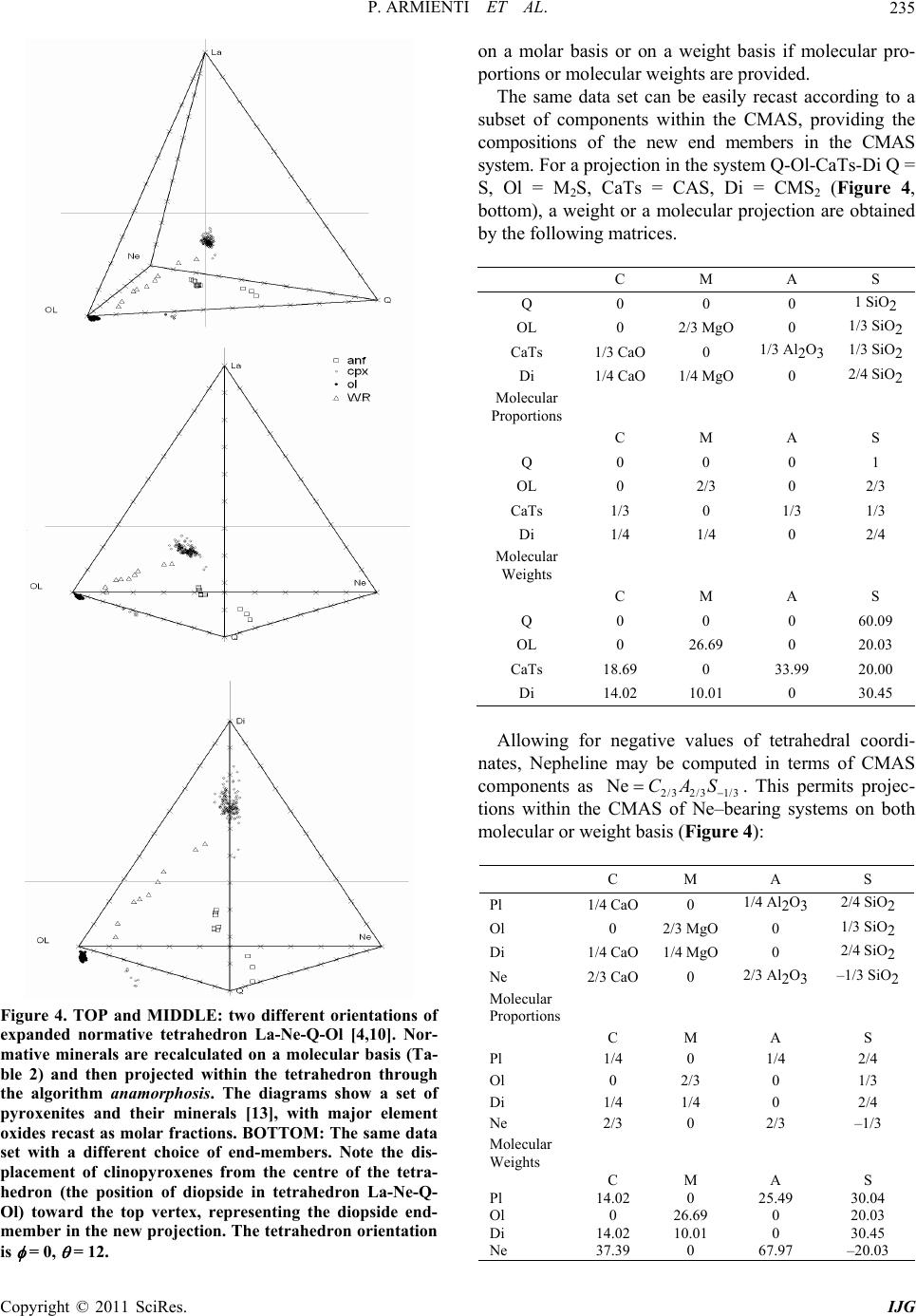

P. ARMIENTI ET AL.235
Figure 4. TOP and MIDDLE: two different orientations of
expanded normative tetrahedron La-Ne-Q-Ol [4,10]. Nor-
mative minerals are recalculated on a molecular basis (Ta-
ble 2) and then projected within the tetrahedron through
the algorithm anamorphosis. The diagrams show a set of
pyroxenites and their minerals [13], with major element
oxides recast as molar fractions. BOTTOM: The same data
set with a different choice of end-members. Note the dis-
placement of clinopyroxenes from the centre of the tetra-
hedron (the position of diopside in tetrahedron La-Ne-Q-
Ol) toward the top vertex, representing the diopside end-
member in the new projection. The tetrahedron orientation
is
 = 0,  = 12.
on a molar basis or on a weight basis if molecular pro-
portions or molecular weights are provided.
The same data set can be easily recast according to a
subset of components within the CMAS, providing the
compositions of the new end members in the CMAS
system. For a projection in the system Q-Ol-CaTs-Di Q =
S, Ol = M2S, CaTs = CAS, Di = CMS2 (Figure 4,
bottom), a weight or a molecular projection are obtained
by the following matrices.
C M A S
Q 0 0 0
1 SiO2
OL 0 2/3 MgO 0
1/3 SiO2
CaTs 1/3 CaO 0
1/3 Al2O3 1/3 SiO2
Di 1/4 CaO 1/4 MgO 0 2/4 SiO2
Molecular
Proportions
C M A S
Q 0 0 0 1
OL 0 2/3 0 2/3
CaTs 1/3 0 1/3 1/3
Di 1/4 1/4 0 2/4
Molecular
Weights
C M A S
Q 0 0 0 60.09
OL 0 26.69 0 20.03
CaTs 18.69 0 33.99 20.00
Di 14.02 10.01 0 30.45
Allowing for negative values of tetrahedral coordi-
nates, Nepheline may be computed in terms of CMAS
components as 2/3 2/31/3 Ne CAS


. This permits projec-
tions within the CMAS of Ne–bearing systems on both
molecular or weight basis (Figur e 4 ):
C M A S
Pl 1/4 CaO0
1/4 Al2O3 2/4 SiO2
Ol 0 2/3 MgO 0
1/3 SiO2
Di 1/4 CaO1/4 MgO 0 2/4 SiO2
Ne 2/3 CaO0
2/3 Al2O3 –1/3 SiO2
Molecular
Proportions
C M A S
Pl 1/4 0 1/4 2/4
Ol 0 2/3 0 1/3
Di 1/4 1/4 0 2/4
Ne 2/3 0 2/3 –1/3
Molecular
Weights
C M A S
Pl 14.02 0 25.49 30.04
Ol 0 26.69 0 20.03
Di 14.02 10.01 0 30.45
Ne 37.39 0 67.97 –20.03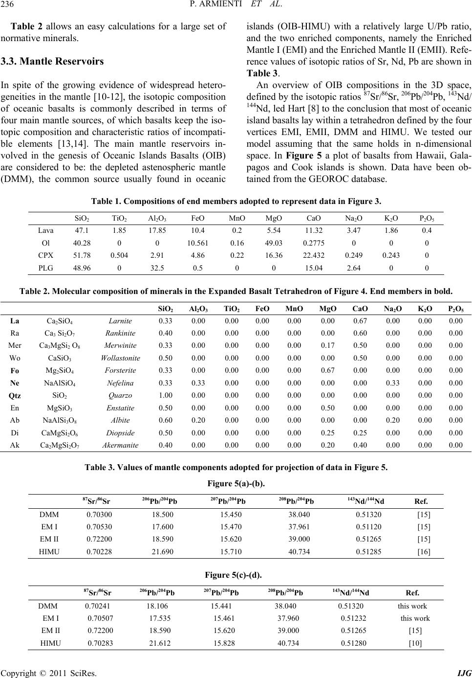

P. ARMIENTI ET AL. 236
Table 2 allows an easy calculations for a large set of
normative minerals.
3.3. Mantle Reservoirs
In spite of the growing evidence of widespread hetero-
geneities in the mantle [10-12], the isotopic composition
of oceanic basalts is commonly described in terms of
four main mantle sources, of which basalts keep the iso-
topic composition and characteristic ratios of incompati-
ble elements [13,14]. The main mantle reservoirs in-
volved in the genesis of Oceanic Islands Basalts (OIB)
are considered to be: the depleted astenospheric mantle
(DMM), the common source usually found in oceanic
islands (OIB-HIMU) with a relatively large U/Pb ratio,
and the two enriched components, namely the Enriched
Mantle I (EMI) and the Enriched Mantle II (EMII). Refe-
rence values of isotopic ratios of Sr, Nd, Pb are shown in
Table 3.
An overview of OIB compositions in the 3D space,
defined by the isotopic ratios 87Sr/86Sr, 206Pb/204Pb, 143Nd/
144Nd, led Hart [8] to the conclusion that most of oceanic
island basalts lay within a tetrahedron defined by the four
vertices EMI, EMII, DMM and HIMU. We tested our
model assuming that the same holds in n-dimensional
space. In Figure 5 a plot of basalts from Hawaii, Gala-
pagos and Cook islands is shown. Data have been ob-
tained from the GEOROC database.
Table 1. Compositions of end members adopted to represent data in Figure 3.
SiO2 TiO2 Al2O3 FeO MnO MgO CaO Na2O K2O P2O5
Lava 47.1 1.85 17.85 10.4 0.2 5.54 11.32 3.47 1.86 0.4
Ol 40.28 0 0 10.561 0.16 49.03 0.2775 0 0 0
CPX 51.78 0.504 2.91 4.86 0.22 16.36 22.432 0.249 0.243 0
PLG 48.96 0 32.5 0.5 0 0 15.04 2.64 0 0
Table 2. Molecular composition of minerals in the Expanded Basalt Tetrahedron of Figure 4. End members in bold.
SiO2 Al2O3 TiO2 FeOMnO MgO CaO Na2O K2O P2O5
La Ca2SiO4 Larnite 0.33 0.00 0.00 0.00 0.00 0.00 0.67 0.00 0.00 0.00
Ra Ca3 Si2O7 Rankinite 0.40 0.00 0.00 0.00 0.00 0.00 0.60 0.00 0.00 0.00
Mer Ca3MgSi2 O8 Merwinite 0.33 0.00 0.00 0.00 0.00 0.17 0.50 0.00 0.00 0.00
Wo CaSiO3 Wollastonite 0.50 0.00 0.00 0.00 0.00 0.00 0.50 0.00 0.00 0.00
Fo Mg2SiO4 Forsterite 0.33 0.00 0.00 0.00 0.00 0.67 0.00 0.00 0.00 0.00
Ne NaAlSiO4 Nefelina 0.33 0.33 0.00 0.00 0.00 0.00 0.00 0.33 0.00 0.00
Qtz SiO2 Quarzo 1.00 0.00 0.00 0.00 0.00 0.00 0.00 0.00 0.00 0.00
En MgSiO3 Enstatite 0.50 0.00 0.00 0.00 0.00 0.50 0.00 0.00 0.00 0.00
Ab NaAlSi3O8 Albite 0.60 0.20 0.00 0.00 0.00 0.00 0.00 0.20 0.00 0.00
Di CaMgSi2O6 Diopside 0.50 0.00 0.00 0.00 0.00 0.25 0.25 0.00 0.00 0.00
Ak Ca2MgSi2O7 Akermanite 0.40 0.00 0.00 0.00 0.00 0.20 0.40 0.00 0.00 0.00
Table 3. Values of mantle components adopted for projection of data in Figure 5.
Figure 5(a)-(b).
87Sr/86Sr 206Pb/204Pb 207Pb/204Pb 208Pb/204Pb 143Nd/144Nd Ref.
DMM 0.70300 18.500 15.450 38.040 0.51320 [15]
EM I 0.70530 17.600 15.470 37.961 0.51120 [15]
EM II 0.72200 18.590 15.620 39.000 0.51265 [15]
HIMU 0.70228 21.690 15.710 40.734 0.51285 [16]
Figure 5(c)-(d).
87Sr/86Sr 206Pb/204Pb 207Pb/204Pb 208Pb/204Pb 143Nd/144Nd Ref.
DMM 0.70241 18.106 15.441 38.040 0.51320 this work
EM I 0.70507 17.535 15.461 37.960 0.51232 this work
EM II 0.72200 18.590 15.620 39.000 0.51265 [15]
HIMU 0.70283 21.612 15.828 40.734 0.51280 [10]

P. ARMIENTI ET AL.237
= 120, = 8, 87Sr/ 86Sr; 206Pb/204Pb; 143Nd/144Nd = 120, = 8, 87Sr/ 86Sr;; 206Pb/204Pb; 208Pb/204Pb;143Nd/144Nd
(a) (b)
= 148, = 8, 87Sr/ 86Sr;; 206Pb/204Pb; = 322,  = 8, 87Sr/ 86Sr;; 206Pb/204Pb;
208Pb/204Pb; 207Pb/204Pb;143Nd/144Nd 208Pb/204Pb; 207Pb/204Pb;143Nd/144Nd
(c) (d)
Figure 5. (a) Three isotope ratios (87Sr/86Sr,206Pb/204Pb, 143Nd/144Nd) were used to define mantle compone nts and plot Hawaii,
Galapagos and Coock Islands basalts and Hawaii mantle xenoliths. (b) The same data set were plotted using the same
tetrahedron orientation but using five isotope compositions (87Sr/86Sr,206Pb/204Pb,207Pb/204Pb, 208Pb/204Pb, 143Nd/144Nd) to
define the HIMU, DMM, EMI and EM II mantle. Data still group in well distinct arrays that can be put in evidence by a
suitable choice of  and  . Values of isotope ratios of mantle components are reported in Table 3, upper part. (c), (d) A
different choice for isotope compositions of mantle components and tetrahedron orientation allows to get a better
representation of regular arrays defined by the data sets. Values adopted for the end members are given in the second part of
table 3. Basalt data from the GEOROC data base.

P. ARMIENTI ET AL. 238
Diagram of Figure 5(a) reveals that points form diffe-
rent clusters in the tetrahedron for the two archipelagos.
Some of the Cook Islands data fall just on the HIMU
component and all data sets appear to point towards
the HIMU component (Figure 5(a)). In particular, it is
possible to observe a branch of the Hawaii data set di-
rected towards an enriched component Figure 5(d)),
while harzburgite mantle xenoliths show an evident im-
print of an EM I end member.
Both Hawaii and Galapagos are widely recognized as
plume-related island chains; thus a plume HIMU com-
ponent should appear to mix with astenospheric mantle
in both island chains, as it results from Figure 5(a),
obtained using tree isotopic ratios.
However, this plotting method may be used to repre- sent
the same data set adopting a larger number of inde-
pendent components, as in Figure 5(b)-(d). The end
members are still defined as HIMU; DMM, EMI and
EMII but using five components (87Sr/86Sr, 206Pb/204Pb,
207Pb/204Pb, 208Pb/204Pb, 143Nd/144Nd ) to plot the same
data set. This allows to observe a different point arrange-
ments: each data set keeps a well distinct trend in every
diagram, but tends to form more dispersed clusters, due
to a larger number of components used to define end
members. A different choice for isotopic compositions of
mantle components and tetrahedron orientation may allow
to get a better representation of regular arrays in the data
sets (Figure 5(c) and (d)). Hawaii data suggest the
mixing between two mantle components, while a plane
arrange- ment suggests that the mixing of three mantle
com- ponents is needed to produce Galapagos basalts.
Values adopted for the new end members are given in
the second part of Table 3.
A suitable choice of end members,  and  allows to
recognize a typical compositional imprint for each mantle
region, in spite of the starting hypothesis of a common
HIMU source depicted in Figure 5(a).
A detailed interpretation of petrogenetic hypotheses is
beyond the purposes of this paper. However, it is evident
how our approach allows an insight, into data sets,
deeper than the simple diagrams in which two isotopic
ratios only are adopted.
4. Conclusions
Our method provides a useful and general way to visua-
lize, in three-dimensional diagrams, data sets charac-
terized by a high number of components. Data are ortho-
gonally projected from the Euclidean space R
n to the
three-dimensional subspace of Rn passing through four
suitable end members, previously chosen. The method
evaluates the tetrahedral coordinates, allowing to map
any point in Rn to the R3 point with the same tetra-
hedral coordinates, obtaining a distorted map (anamor-
phosis) of a perhaps highly irregular tetrahedron in Rn
into a regular tetrahedron in R3. This procedure ensures
normalization of data and allows to use components
whose numerical values may differ in the order of mag-
nitude.
End member physical mixtures (convex combinations)
are represented by points within the tetrahedron and the
methods developed for the study of “constant sum” sets
[5,8] may be applied for the interpretation of data. How-
ever, our projection method also allows the represen-
tation of natural compositions laying outside the Rn tetra-
hedron as linear (non convex) combinations of the end
members, plotting them outside the 3D tetrahedron. If
these points fall far from the tetrahedron, a different
choice of end members may be accomplished to find a
tetrahedron containing them.
A final projection from R3 to the graphic plane plots
the diagram; suitable orientation of the tetrahedron in the
plot reveals 1D and 2D arrays, corresponding to binary
or ternary mixtures. Animated rotation of the diagram
may be easily obtained and allows a fast and effective
overview of data sets. The use of mineral and rock ana-
lyses to define end members ensures the possibility of
the geometrical solution of mass balance problems. The
obvious application of this kind of plots may be found in
experimental petrology for the representation of com-
positions of complex systems like the normative Basalt
tetrahedron or the CMAS system, computed on a
weight% or molecular basis. This kind of projections
also allows to explore multidimensional data sets, like
those characterizing the isotope systematic of magmas
and their incompatible element ratios.
5. References
[1] P. Armienti, “TETRASEZ an Interactive Program in BA-
SIC to Perform Tetrahedral Diagrams,” Computer &
Geosciences, Vol. 12, No. 2, 1986, pp. 229-241.
doi:10.1016/0098-3004(86)90010-5
[2] R. O. Sack, D. C. Walker and I. S. E. Carmichael, “Ex-
perimental Petrology of Alkalic Lavas: Constraints on
Cotectics of Multiple Saturation in Natural Basic Liq-
uids,” Contributions to Mineralogy and Petrology, Vol.
96, No. 1, 1987, pp. 1-23.
doi:10.1007/BF00375521
[3] M. J. O’Hara, “The Bearing of Phase Equilibria Studies
on the Origin and Evolution of Basic and Ultrabasic
Rocks,” Earth-Sci ence Rev iews, Vol. 4, 1968, pp. 69-133.
doi:10.1016/0012-8252(68)90147-5
[4] H. S. J. Yoder and C. E. Tilley, “Origin of Basalt Magma:
An Experimental Study of Natural and Synthetic Rock
Systems,” Journal of Petrology, Vol. 3, No. 3, 1962, pp.
342-532.
[5] J. Aitchison, “The Statistical Analysis of Compositional

P. ARMIENTI ET AL.239
Data,” Chapman and Hall, London, 1986, p. 416.
[6] C. J. Allègre, B. Hamelin, A. Provost and B. Dupré,
“Topology of Isotopic Multispace and Origin of Mantle
Chemical Etherogenities,” Earth and Planetary Sience
Letters, Vol. 81, 1986, pp. 319-337.
[7] P. Armienti, S. Tonarini, F. Innocenti and M. D’Orazio,
“Mount Etna Pyroxene as Tracer of Petrogenetic Proc-
esses and Dynamics of the Feeding System,” In: L. Bec-
caluva, G. Bianchini, M. Wilson, Eds., Volcanism in the
Mediterranean and Surrounding Regions, Geological So-
ciety of America, Special Paper, Vol. 418, 2007, pp.
265-276.
[8] J. F. Schairer and H. S. Yoder Jr., “Crystal and Liquid
Trends in Simplified Alkali Basalts,” Carnegie Institution
of Washington, Vol. 63, 1964, pp. 65-75.
[9] C. Perinelli, P. Armienti and L. Dallai, “Thermal Evolu-
tion of the Lithosphere in a Rift Environment as Inferred
from the Geochemistry of Mantle Cumulates. Northern
Victoria Land, Antarctica,” Journal of Petrology, Vol. 52,
No. 4, 2011, pp. 665-690.
doi:10.1093/petrology/egq099
[10] S. Hart, E. H. Hauri, L. A. Oschmann and J. A. White-
head, “Mantle Plumes and Entrainment: Isotopic Evi-
dence,” Science, Vol. 256, No. 5056, 1992, pp. 517-520.
doi:10.1126/science.256.5056.517
[11] E. Hauri and S. R. Hart, “Rhenium Abundances and Sys-
tematics in Oceanic Basalts,” Chemical Geology, Vol. 13,
No. 1-4, 1997, pp. 185-205.
doi:10.1016/S0009-2541(97)00035-1
[12] P. Armienti and D. Gasperini, “Do We Really Need Man-
tle Components to Define Mantle Composition?” Journal
of Petrology, Vol. 48, No. 4, 2007, pp. 693-709.
doi:10.1093/petrology/egl078
[13] J. A. Martìn-Fernàndez, C. Barcelò-Vidal and V. Paw-
lowsky-Glahn, “Dealing with Zeros and Missing Values
in Compositional Data Sets Using Nonparametric impu-
tation,” Mathematical Geology, Vol. 35, No. 3. 2003, pp.
45-54.
[14] S. S. Sun and W. F. McDonough, “Chemical and Isotopic
Systematics of Oceanic Basalts: Implications for Mantle
Composition and Processes,” In: A. D. Saunders and M. J.
Norry, Eds., Magmatism in Ocean Basins, Geological
Society Special Publication, London, 1989, pp. 313-345.
[15] A. D. Saunders, M. J. Norry and J. Tarney, “Origin of
MORB and Chemically Depleted Mantle Reservoirs:
Trace Element Constraints,” Journal of Petrology, Vol. 1,
No. 1, 1988, pp. 414-445.
[16] D. J. Chaffey, R. A. Cliff and B. M. Wilson, “Charac-
terization of the St. Helena Magma Source,” In: A. D.
Saunders and M. J. Norry Eds., Magmatism in Ocean Ba-
sins, Geological Society Special Publication, London,
Vol. 42, 1989, pp. 257-276.