Received 2 August 2015; accepted 28 September 2015; published 12 October 2015

ABSTRACT

Parameter estimation by maximizing the marginal likelihood function in generalized linear mixed models (GLMMs) is highly challenging because it may involve analytically intractable high-dimen- sional integrals. In this paper, we propose to use Quasi-Monte Carlo (QMC) approximation through implementing Newton-Raphson algorithm to address the estimation issue in GLMMs. The random effects release to be correlated and joint mean-covariance modelling is considered. We demonstrate the usefulness of the proposed QMC-based method in approximating high-dimensional integrals and estimating the parameters in GLMMs through simulation studies. For illustration, the proposed method is used to analyze the infamous salamander mating binary data, of which the marginalized likelihood involves six 20-dimensional integrals that are analytically intractable, showing that it works well in practices.

Keywords:

Generalized Linear Mixed Models, Correlated Random Effects, Quasi-Monte Carlo, Mean-Covariance Modelling, High-Dimensional Integrals, Newton-Raphson Method

Subject Areas: Mathematical Statistics

1. Introduction

McCullagh and Nelder (1989) [1] analyzed a challenging salamander mating binary data set which was conducted on two geographically isolated populations, Roughbutt (RB) and Whiteside (WS), in three experiments (one in summer 1986 and two in fall 1986). The question of interest is to determine whether or not certain barriers to interbreeding have evolved over time in geographically isolated populations. The second question is to determine whether or not heterogeneity between individuals (females and males) exists. The RB and WS populations are ideal for these experiments because salamanders would never meet those from different population in their natural environment, so that there are two closed groups in each experiment. Each group involved five females and five males from each population. Each female mated with six males, three from each population. So each closed group resulted in sixty correlated binary observations (1 for successful mating; 0 for failed mating). Therefore, the binary data set is crossed, balanced (as each female mated with a total of six males and vice verse) and incomplete (as each female mated with just three out of a possible five males, and vice verse). The data can be analyzed by using a specific generalized linear mixed model.

Generalized linear mixed models (GLMMs) are very useful for non-Gaussian correlated or clustered data and widely applied in many areas including epidemiology, ecological, and clinical trials. Parameters estimation in GLMMs is, however, very challenging, and correlated binary data is even more difficult to analyze than continuous data. This is because the marginalized likelihood function, obtained by integrating out multivariate random effects from the joint density function of the responses and random effects, is in general analytically intractable. For example, the likelihood function for the pooled salamander mating data described above involves six 20-dimensional integrals which are analytically intractable. In the literature, the marginalized likelihood function was considered by two typical methods: a) analytical Laplace approximation to integrals: This is represented by the work of Breslow and Clayton (1993) [2] who developed the penalized quasi-likelihood (PQL) estimation. Unfortunately, approaches based on Laplace approximation may yield biased estimates of variance components, particularly for modeling correlated binary data. This difficulty has stimulated a number of alternative approaches. For example, Lin and Breslow (1996) [3] proposed a corrected penalized quasi-likelihood, and Lee and Nelder (2001) [4] developed hierarchical generalized linear models (HGLMs) procedure; b) numerical techniques to approximate the likelihood function and estimate the parameters: Karim and Zeger (1992) [5] developed a Bayesian approach with Gibbs sampling for GLMMs, but its computational efforts may be computationally intensive. Monte Carlo Expectation-Maximization (MCEM) and Monte Carlo Newton-Raphson (MCNR) algorithms were proposed to approximate the maximum likelihood estimates in GLMMs by McCulloch (1994, 1997) [6] [7] . However, iterations of MCEM and MCNR do not always converge to the global maximum and are also very computationally intensives for high-dimensional problems (Chan, Kuk and Yam, 2005) [8] . Pan and Thompson (2003, 2007) [9] [10] developed Gauss-Hermite Quadrature (GHQ) approach and Quasi-Monte Carlo (QMC) approximation. Aleid and Pan (2008) [11] used Randomized Quasi-Monte Carlo (RQMC) to solve the integration problem in GLMMs. It is noted that most of the work above assume that random effects in GLMMs, which characterize the heterogeneity among individuals, are mutually independent and normally distributed.

However, these assumptions may not always hold due to the likely correlation of random effects, for instance. At least, the independence assumption of random effects should be testable. Misspecification of random effects covariance structure may yield inefficient estimates of parameters and can cause the problem of biased estimates of variance components, making statistical inferences for GLMMs unreliable. In this paper, we release the assumption of independence for random effects and aim to develop a new methodology which can model the covariance structures of random effects in GLMMs. Covariance modeling strategy based on a modified Cholesky decomposition is studied within the framework of GLMMs. The paper is organized as follows. GLMMs and the marginalized Quasi-likelihood are briefly reviewed in Section 2. The QMC approximation, the simplest good point set and analytical form of the MLEs for GLMMs are discussed in Section 3. Covariance modeling strategy through a modified Cholesky decomposition is described in Section 4. In Section 5, the salamander data set is analyzed as an example for illustration of the use of the new method. Simulation studies with the same design protocol as the salamander data are conducted in Section 6. Discussions on the related issues and further studies are presented in Section 7.

2. Generalized Linear Mixed Models

Let denote the observed responses. Assume that is the row of design matrix X; is the fixed effects parameter; is the row of the second design matrix Z; and b is the random effects.

The GLMMs are of the form

, (1)

where is a monotonic and differentiable link function. Given random effects b, the responses are independent and follow an exponential family of distributions with the density

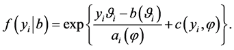(2)

The conditional mean and variances, given random effects b, are given by and

, respectively, where is a prior weight, is an overdispersion scalar,

is the so-called natural parameter, and are the first- and second-derivatives of, and is the known variance function (McCullagh and Nelder, 1989) [1] .

When the linear predictor is identical to, i.e., , GLMMs are said to have a canonical link function. In this article we assume the model has a canonical link function, although the proposed method can be extended straightforwardly to non-canonical link functions. Like generalized linear models (GLMs), the choice of canonical link function depends on the distribution of data. For example, for binary responses the canonical link function is the logit function, which takes the form

. (3)

Note q-dimensional random effects b are assumed to be normally distributed with mean 0 and positive definite variance-covariance matrix, where is an m-variant vector of variance components.

Quasi-likelihood function of the fixed effects and variance components in GLMMs, also called marginal quasi-likelihood function, can be expressed by

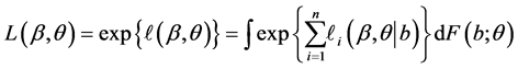, (4)

where

(5)

so that

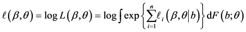(6)

is the conditional log quasi-likelihood of and, given random effects b (Breslow and Claybon, 1993) [2] . F(b; θ) is CDF of random effect b.

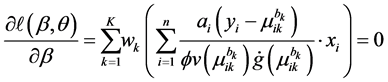
It is challenging to calculate the maximum likelihood estimates (MLEs), and, that maximize the above conditional log quasi-likelihood, because it likely involves high-dimensional integrals which are analytically intractable. This computational problem becomes more severe when random effects are multivariate and correlated.

3. Quasi-Monte Carlo Integration and Estimation

3.1. Monte Carlo (MC) Integration

In this section, Quasi-Monte Carlo (QMC) approach is used to approximate high dimensional integrals. The traditional Monte Carlo (MC) method is outlined first as follow. Let be an integrable function over the q-dimensional unit cube. Without loss of generality, we consider the following integrals

(7)

Assume K independent random samples are drawn from the uniform distribution on and used to approximate the integral (7) through

(8)

According to the strong law of large number, the approximation converges to the true value of the integral with probability one as. The central limit theorem assures that the distribution of converges to normal distribution with mean and variance as. The convergence rate for MC integration has an order, which is independent of the dimension of integral.

Since the rate of convergence is independent of q, the MC approximation seems to be very appealing. However, the MC algorithm has some serious drawbacks (see, e.g., Niederreiter, 1992 [12] ; Spanier and Maize, 1994 [13] ). One of these deficiencies is that even though the rate of convergence is independent of the dimension, the convergence is very slow. On the other hand, it may suffer from the problem of generating genuinely random samples. Instead, pseudo-random samples are generated and used to approximate the integral (Traub and Wozniakowski, 1992 [14] ). It is also noted that the MC method only provides probabilistic error bounds, which is not a desirable as it does not guarantee reliable estimation results. As an alternative to the MC methods, Quasi- Monte Carlo approximation method is considered.

3.2. Quasi-Monte Carlo Method and Lattice Rule

Quasi-Monte Carlo (QMC) sequences are a deterministic alternative to Monte Carlo sequences (Niderreiter, 1992). In contrast to MC sequences, QMC sequences have a property that they are uniformly distributed on the unit cube. Thus, QMC approximation has the same equation as (8) but the MC random samples are replaced by deterministic samples that are uniformly distributed on the domain. Uniformity of sequences is measured by means of discrepancy, and for this reason QMC sequences are also called low-discrepancy sequences. Note the Koksma-Hlawka inequality

(9)

where and are given in (7) and (8), respectively, is the variation of in the sense of Hardy and Krause (Fang and Wang, 1994, p. 64 [15] ) and is the star discrepancy that measures the uniformity of distribution of a finite point set, see Fang and Wang (1994) for the details. The Koksma-Hlawka inequality implies that the absolute integration error is bounded by the star discrepancy of multiplied by the variation. Since the latter is fixed as along as the function f is given, the absolute integration error can be minimized by carefully choosing the integration nodes. It can be shown

that the absolute integration error has an order, so that integration nodes should be

chosen such that their start discrepancy is close to. For large K, this rate of convergence is considerably faster than the crude MC approach whose error is bounded to. More details regarding to the superiority of the QMC method over the MC method can be found in Morokoff and Caflisch (1995) [16] , and Fang and Wang (1994) [15] .

In the QMC approach, there are many good algorithms for generating such integration nodes. One set of such integration nodes is called good point set and discussed below.

3.3. Good Point (GP) Set

Denote a good point by where is a hy-

percube. The set consists of the first K points of the set, where

represents the fractional part of for. In practice, the following form of the good point is quite common to use,

, (10)

where is a prime number and,. For example, they can be chosen as the first q primes.

3.4. MLE via QMC Approximation

Suppose is a GP set. When the QMC method is applied to the marginal quasi-likelihood function (6), we obtain

, (11)

where is the inverse of, the CDF of random effects b, and is the square root of, for

example, it can be taken as the Cholesky decomposition of or eigenvalue-eigenvector decomposition.

Let, so that and where is

the inverse function of the link function. The maxima of with respect to and is the solution of the score equations

, (12)

(13)

where, and is a weight for the kth point given by

(14)

Note that the weight given above is a function of and, i.e., , which should be taken into account when calculating the second-order derivatives.

In general, the score equations in (12)-(13) have no analytical solutions for and. We then propose to use Newton-Raphson algorithm to update the solutions, though calculation of Hessian matrix is somewhat difficult. In Appendices A and B of this paper, we report the detailed calculation of Hessian matrix. When the difference between and, and/or the difference between and, is small enough, the maximum likelihood estimates of β and are achieved. At convergence, the asymptotic variance-covariance matrix of the MLE is also obtained straightforwardly through the inverse of Hessian matrix.

4. Modeling of Covariance Structures of Random Effects

Misspecification of covariance structures of random effects may cause problems of inefficient estimates of parameters in GLMMs. In some circumstances, it may lead to biased estimates of the parameters. Hence, in this paper we propose to model the covariance structure of random effects in GLMMs, rather than specify a structure to the covariance matrix of random effects b. In a spirit of Pourahmadi (1999; 2000) [17] [18] , we consider a modified Cholesky decomposition of, instead of, for obtaining a statistically meaningful parametrization of the covariance matrix. The modified Cholesky decomposition removes three difficulties arising in modeling covariance structures: a) covariance matrix is usually positive definite; b) covariance matrix may be of large size; and c) the parametrization has to take into account of computational efficiency and statistical interpretation. In the past decade, an increasing attention to the decomposition was paid by many statisticians including Daniels and Pourahmadi (2002) [19] , Daniels and Zhao (2003) [20] , Smith and Kohn (2002) [21] , Pan and MacKenzie (2003) [22] , and Ye and Pan (2006) [11] among others. The key of the modified Cholesky decomposition is that a symmetric matrix is positive definite if and only if there exist a unique unit lower triangular matrix T with 1’s as its diagonal entries, and a unique diagonal matrix D with positive diagonal entries, such that

, (15)

where

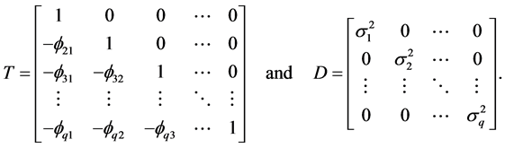(16)

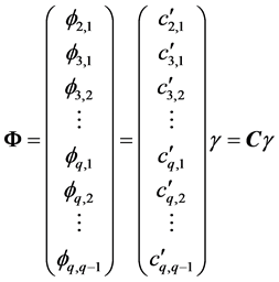
Thus, and. The modified Cholesky decomposition of offers a simple unconstrained and statistically meaningful reparametrization of the covariance matrix. T and D are easy to compute and interpret statistically: the below-diagonal entries of T are the negative of autoregressive coefficients (ACs), say, in the autoregressive model

, (17)

where is the kth component of the vector of random effects b. In other words, is the linear least squares predictor of based on its predecessors. On the other hand, the diagonal entries of D are the in-

novation variances (IVs), i.e., where. Obviously, if

. Let, then so that.

In a spirit of Pourahmadi (1999) [17] , we propose to model the ACs and the logarithm of the IVs using linear regression models

(18)

where and are covariates, and and are low-dimensional parameter vectors. Hence, the parameter vector of variance components is.

5. Salamander Data Analysis

Assume that is the outcome for the mating of the ith female salamander with the jth male. Consider the following logit mixed model for each experiment

(19)

where is the conditional probability of successful mating of the pair,

with if the female comes from WS, and 0 otherwise. Similarly, if the male comes from WS, and 0 otherwise.

Note that each experiment involves 40 salamanders so that the log-likelihood function for each experiment involves one 40-dimensional integral. It can be further reduced to the sum of two 20-dimensional integrals due to the block design of the two closed groups, see Karim and Zeger (1992) [5] and Shun (1997) [23] for more details about the design. When the three-experiment data sets are pooled as those in model (19), the log-likelihood function is a sum of six 20-dimensional integrals which are analytically intractable, so that the MLEs of the fixed effects and variance components become extremely difficult to calculate. In the literature, several analytical and numerical approximations were proposed to overcome the difficulties in evaluating the log-likelihood function. Examples include MCMC method by Karim and Zeger (1992) [5] , MCEM algorithm by McCulloch (1994) [6] and PQL estimation by Breslow and Clayton (1993) [2] . However, all the literature work assumed that the covariance matrix of random effects has certain structures.

We now apply the proposed covariance modeling method to the salamander mating data. Note. We consider the following model for the autoregressive coefficients,

(20)

where is the negative of the th element of the lower triangular matrix T in the modified Cholesky decomposition (;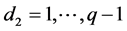), so that is a -dimensional vector. is an design matrix with rows

(21)

where if the and salamanders come from different genders, and 0 otherwise. Similarly, if the and salamanders come from different districts, and 0 otherwise. γ is an -variant vector of parameters.

The model for the innovation variances is

(22)

where is an q-variant vector. is an design matrix with rows

(23)

where if the salamander is female, and 0 otherwise. Similarly, if the salamander comes from WS, and 0 otherwise. Note λ is an -variant vector of parameters and are the diagonal elements of the matrix D in the modified Cholesky decomposition.

The pooled data are now analyzed using the proposed QMC approach. The MLEs of the fixed effects and variance components in the model are calculated. Specifically, we implement the simplest QMC points, square root sequences, to approximate the 20-dimensional analytically intractable integrals. A set of 20-dimensional points on the unit cube are generated to approximate the six 20-dimensional integrals in the marginalized log-likelihood function. We then use Newton-Raphson algorithm to maximize the approximated log-likelihood function for the pooled data.

Note that the covariance modeling for, the covariance matrix of random effects, uses parameters for modeling of the autoregressive coefficients and parameters for the innovation variances. By using the joint mean-covariance modeling strategy we can model the structure of and estimate the covariance matrix without specifying a covariance structure to. This avoids the problem of misspecification of covariance structures. In addition, the number of parameters in reduces from to, which avoids high-dimensional problems of covariance estimation when q is large. Finally, the modeling strategy based on the modified Cholesky decomposition guarantees that the resulting estimate of is positive definite.

We code our programme in FORTRAN and run on a PC Pentium (R) 4 PC (CPU 3.20 GHz). We choose the PQL estimate as the starting value of, i.e., , and zero as for. Table 1 reports the numerical results when increasing the number of integration nodes generated by the square root sequences. From Table 1, we can see that the simplest GP point set works reasonably well for calculating the MLEs of the parameters in models (19), (20) and (22). The results show that the maximized

log-likelihood changes very little when the number of integration nodes increases from 10,000 to 100,000, implying that any number of the points between these numbers would be fine to obtain reasonably good estimates of the parameters. On the other hand, the parameter estimates using these sequences become stable quickly. We notice that the integral space is 20-dimensional so that the points are very sparse even if the number of the QMC points increases to. In the meantime, the algorithm gets convergence very quickly and it only takes a few of iterations to achieve the convergence. In the case of using integration nodes, for example, our Fortran code takes only several minutes to obtain the estimation results.

It is noted that in the autoregressive coefficients model, the estimates of, including, , and, are all very close to zero and not statistically significant. Therefore, the estimates of the autoregressive coefficients can be regarded as zero. On the other hand, in the model of the log-innovation variances, the estimates of the regression parameters, except, are not statistically significant.

In other words, T is an identity matrix and D is a diagonal matrix with an identical element on diagonals, implying where. Hence, it is concluded that the random effects in the modeling of the salamander mating data are uncorrelated, and so there is no heterogeneity between the female and male salamanders.

By comparing the numerical results of the QMC estimation approach with the literature work, we find that they are quite close to those made by Gibbs sampling method. But the QMC method has much light computational loads and easy to use for practitioners. This is because Gibbs sampling method involves multiple draws of random samples and needs more experience, for instance, in specifying prior distributions of parameters, etc., whereas the QMC approximation method does not need such specifications. Also, Gibbs sampling may be very slow in obtaining the parameter estimates. On the other hand, the PQL approach gives very biased estimates of the variance components for modeling clustered binary data, as reported by many authors including Breslow and Clayton (1993) [2] , Breslow and Lin (1995) [24] , Booth and Hobert (1999) [25] and Aiken (1999) [26] .

6. Simulation

In this section, we carry out simulation studies to assess the performance of the proposed QMC estimation method in GLMMs. In the simulation studies we consider the logistic model (19) and use the same protocol of design as the real salamander mating experiment, resulting in 360 correlated binary observations. We run 100 simulations and calculate the average of the parameter estimates over the 100 simulations. The log-likelihood function for each simulated data set involves six 20-dimensional integrals that are analytically intractable.

We generate integration nodes on the unit cube using the square root sequences. We then use those integration nodes to approximate the integrated log-likelihood as the one given in (11), and use Newton-Raphson algorithm to maximize the approximated log-likelihood function. The true fixed effects are chosen to be, which is quite close to the one obtained in the real data analysis presented in the previous section. In the real data analysis there is no heterogeneity between female and male, but in our simulation studies we choose for modeling the ACs and for the IVs in order to assess the performance of the proposed method when heterogeneity occurs. The starting values of the parameters are chosen to be the parameter estimates from the real data analysis. The estimation results of the simulation studies are summarized in Table 2, which presents the average of the parameter estimates over 100 replications and their standard errors as well.

From Table 2 it is clear that the proposed QMC approach is able to produce reasonably good estimates of parameters in GLMMs even if there are heterogenous random effects. The estimates of the fixed effects and variance components, based on the average of 100 simulation results, are quite close to the true values of the parameters. It implies that the proposed QMC approach with covariance modeling strategy works well in estimating parameters in GLMMs with correlated random effects.

7. Discussions

We have studied the performance of using QMC approach to calculate the MLEs of the fixed effects and variance components in GLMMs with correlated random effects. We proposed to use Newton-Raphson algorithm to calculate the parameter estimates. The marginalized log-likelihood function that is in general analytically intractable is approximated well through the use of the simplest QMC points, i.e., square root sequences. We also addressed the issue of covariance modelling for random effects covariance matrix through a modified Cholesky decomposition. As a result, pre-specification of covariance structures for random effects is not necessary and misspecification of covariance structures is thus avoided. The score function and observed information matrix are calculated and expressed in analytically closed forms, so that the algorithm can be implemented straightforwardly. The performance of the proposed method was assessed through real salamander mating data analysis and simulation studies. Even though the marginalized log-likelihood function in the numerical analysis involves six 20-dimensional analytically intractable integrals, the QMC square root sequence approximation performs very well.

In general, a practical issue for the use of the QMC points is the choice of the number of integration nodes. Pan and Thompson (2007) [10] suggested to increase the number of integration points gradually until the estimation results become relatively stable. This is exactly what we have done in the numerical analysis displayed in Table 1.

Acknowledgements

We thank the editors and the reviewers for their comments. This research is funded by the National Social Science Foundation No.12CGL077, National Science Foundation granted No.71201029, No.71303045 and No.11561071. This support is greatly appreciated.

Cite this paper

Yin Chen,Yu Fei,Jianxin Pan, (2015) Quasi-Monte Carlo Estimation in Generalized Linear Mixed Model with Correlated Random Effects. Open Access Library Journal,02,1-16. doi: 10.4236/oalib.1102002

References

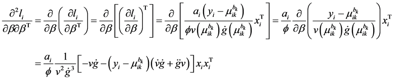
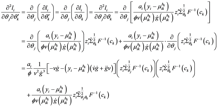
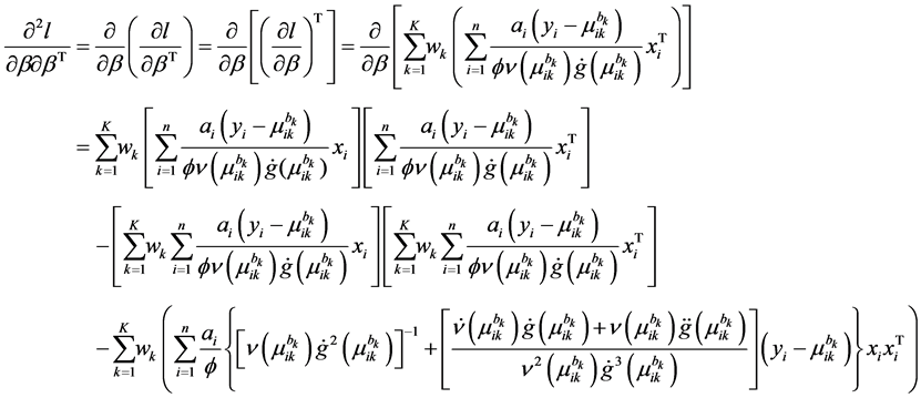
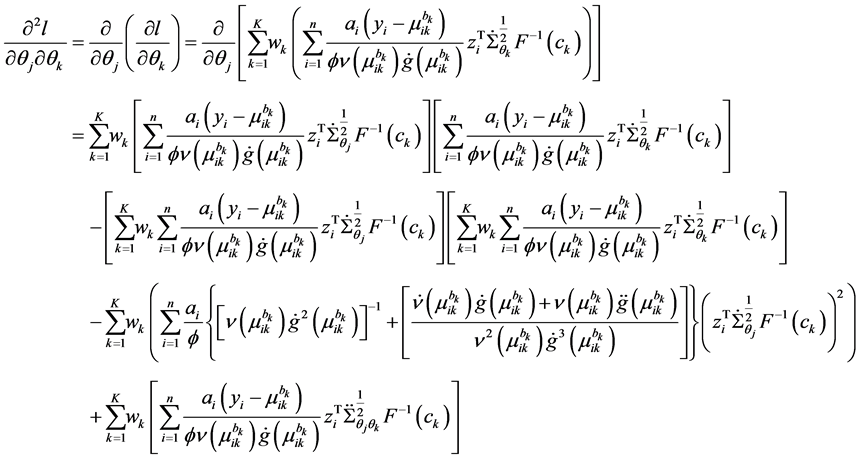
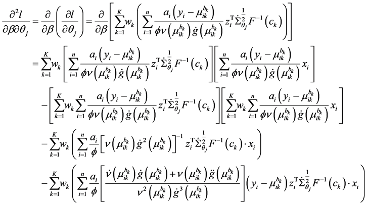
Appendix A: Second-Order Derivatives of Log-Likelihood

The second-order derivatives of log-likelihood function is given by

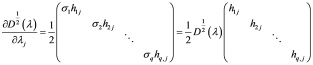
Appendix B: MLEs for Covariance Modeling

The first and second derivative of respect to and are:

(24)

(25)

(26)

is introduced for the purpose of calculation for, and. Note that the ma-

trix looks similar to the matrix T, but opposite sign for the lower triangular elements.

(27)

Every element in was rearranged into a response vector, such that, i.e.,

(28)

We can put the j^th column of C into a lower triangular matrix like. So we have matrices. The element in (28) can be put into the place in the j^th matrix. For the j^th matrix, , we

have the relationship where, and.

The above relationship is a one-to-one correspondence between i and. So and in (28) can be also expressed as

(29)

is a lower triangular matrix with 1’s as diagonal entries, so that, and

are all lower triangular matrices. Denote where

(30)

The first derivative can be calculated as

(31)

where is a lower triangular matrix with 0’s as diagonal entries and as the entries below diagonal.

The second derivative can be calculated as

(32)

(33)

because of,. We also have

(34)

(35)

(36)

where

(37)

(38)

(39)

(40)

NOTES

^*Corresponding author.

References

- 1. McCulloch, P. and Nelder, J.A. (1989) Generalized Linear Models. 2nd Edition, Chapman and Hall, London.
http://dx.doi.org/10.1007/978-1-4899-3242-6 - 2. Breslow, N.E. and Clayton, D.G. (1993) Approximate Inference Ingeneralized Linear Mixed Models. Journal of the American Statistical Association, 88, 9-25.
- 3. Lin, X. and Breslow, N.E. (1996) Bias Correction in Generalized Lnear Mixed Models with Multiple Components of Dispersion. Journal of the American Statistical Association, 91, 1007-1016.
http://dx.doi.org/10.1080/01621459.1996.10476971 - 4. Lee, Y. and Nelder, J.A. (2001) Hierrarchical Generalized Linear Models: A Synthesis of Generalized Linear Models, Random Effect Models and Structured Dispersions. Biometrika, 88, 987-1006.
http://dx.doi.org/10.1093/biomet/88.4.987 - 5. Karim, M.R. and Zeger, S.L. (1992) Generalized Linear Models with Random Effects; Salamnder Mating Revisited. Biometrics, 48, 681-694.
http://dx.doi.org/10.2307/2532317 - 6. McCulloch, C.E. (1994) Maximum Likelihood Variance Components Estimation for Binary Data. Journal of the American Statistical Association, 89, 330-335.
http://dx.doi.org/10.1080/01621459.1994.10476474 - 7. McCulloch, C.E. (1997) Maximum Likelihood Algorithms for Generallized Linear Mixed Models. Journal of the American Statistical Association, 92, 162-170.
http://dx.doi.org/10.1080/01621459.1997.10473613 - 8. Chan, J.S., Kuk, A.Y. and Yam, C.H. (2005) Monte Carlo Approximation through Gibbs Output in Generalized Linear Mixed Models. Journal of Maltivariate Analysis, 94, 300-312.
http://dx.doi.org/10.1016/j.jmva.2004.05.004 - 9. Pan, J. and Thompson, R. (2003) Gauss-Hermite Quadrature Approximation for Estimation in Generalised Linear Mixed Models. Computational Statistics, 18, 57-78.
- 10. Pan, J. and Thompson, R. (2007) Quasi-Monte Carlo Estimation in Generalized Linear Mixed Models. Computational Statistics and Data Analysis, 51, 5765-5775.
http://dx.doi.org/10.1016/j.csda.2006.10.003 - 11. Ye, H. and Pan, J. (2006) Modelling Covariance Structures in Generalized Estimating Equations for Longitudinal Data. Biometrika, 93, 927-941.
http://dx.doi.org/10.1093/biomet/93.4.927 - 12. Niederreiter, H. (1992) Random Number Generation and Quasi-Monte Carlo Methods. SIAM, Philadelphia.
http://dx.doi.org/10.1137/1.9781611970081 - 13. Spanier, J. and Maize, E. (1994) Quasi-Random Methods for Estimating Integrals Using Relatively Small Samples. SIAM Review, 36, 19-44.
http://dx.doi.org/10.1137/1036002 - 14. Traub, J.F. and Wozniakowski, H. (1992) The Monte Carlo Algorithm with Pseudorandom Generator. Mathematics of Computation, 58, 323-339.
http://dx.doi.org/10.1090/S0025-5718-1992-1106984-4 - 15. Fang, K.T. and Wang, Y. (1994) Number-Theoretic Methods in Statistics. Chapman and Hall, London.
http://dx.doi.org/10.1007/978-1-4899-3095-8 - 16. Morokoff, W.J. and Caflisch, R.E. (1995) Quasi-Monte Carlo Integration. Journal of Computational Physics, 122, 218-230.
http://dx.doi.org/10.1006/jcph.1995.1209 - 17. Pourahmadi, M. (1999) Joint Mean-Covariance Models with Applications to Longitudinal Data: Unconstrained Parameterization. Biometrika, 86, 677-690.
http://dx.doi.org/10.1093/biomet/86.3.677 - 18. Pourahmadi, M. (2000) Maximum Likelihood Estimation of Generalised Linear Models for Multivariate Normal Covariance Matrix. Biometrika, 87, 425-435.
http://dx.doi.org/10.1093/biomet/87.2.425 - 19. Daniels, M.J. and Pourahmadi, M. (2002) Bayesian Analysis of Covariance Matrices and Dynamic Models for Longitudinal Data. Biometrika, 89, 553-566.
http://dx.doi.org/10.1093/biomet/89.3.553 - 20. Daniels, M.J. and Zhao, Y.D. (2003) Modelling the Random Effects Covariance Matrix in Longitudinal Data. Statistics in Medicine, 22, 1631-1647.
http://dx.doi.org/10.1002/sim.1470 - 21. Smith, M. and Kohn, R. (2002) Parsimonious Covariance Matrix Estimation for Longitudinal Data. Journal of the American Statistical Association, 97, 1141-1153.
http://dx.doi.org/10.1198/016214502388618942 - 22. Pan, J. and MacKenzie, G. (2003) On Modelling Mean-Covariance Structures in Longitudinal Studies. Biometrika, 90, 239-244.
http://dx.doi.org/10.1093/biomet/90.1.239 - 23. Shun, Z. (1997) Another Look at the Salamander Mating Data: A Modified Laplace Approximation Approach. Journal of the American Statistical Association, 92, 341-349.
http://dx.doi.org/10.1080/01621459.1997.10473632 - 24. Breslow, N.E. and Lin, X. (1995) Bias Correction in Generalised Linear Mixed Models with a Single-Component of Dispersion. Biometrika, 82, 81-91.
http://dx.doi.org/10.1093/biomet/82.1.81 - 25. Booth, J.G. and Hobert, J.P. (1999) Maximizing Generalized Linear Mixed Model Likelihoods with an Automated Monte Carlo EM Algorithm. Journal of the Royal Statistical Society, B, 61, 265-285.
http://dx.doi.org/10.1111/1467-9868.00176 - 26. Aitken, M. (1999) A General Maximum Likelihood Analysis of Variance Components in Generalized Linear Models. Biometrics, 55, 117-128.
http://dx.doi.org/10.1111/j.0006-341X.1999.00117.x