International Journal of Geosciences, 2011, 2, 286-292
doi:10.4236/ijg.2011.23031 Published Online August 2011 (http://www.SciRP.org/journal/ijg)
Meridional Asymmetries in Forced Beta-Plane Turbulence
Iordanka N. Panayotova
Old Dominion University, Department of Mathematics and Statistics, Norfolk, United States
Received March 10, 2011; revised April 18, 2011; accepted June 4, 2011
Abstract
Forced geostrophic turbulence on the surface of a rotating sphere (so called β-plane turbulence) is simulated
trough the use of the β-SQG+1 numerical model. Domain occupied by the fluid has a channel geometry with
512 by 256 grid points, periodic boundary conditions in x-direction and rigid boundaries in y-direction.
Random forcing is applied at high wave-numbers in the spectral space. To better understand eddies dynamics
we simulate both regimes, with and without stochastic forcing, starting from identical initial conditions. Di-
rect numerical simulations exhibit different dynamical properties in different regimes. In the freely evolving
case, a wave term that competes with inertia on large-scales (added as a result of the β-effect) produces high
meridional asymmetries in the eddies spatial and time scales. This asymmetry is added to the standard for the
β-plane turbulence zonal asymmetry. In the forced regime there is not only anisotropy in the eddies deforma-
tion radius, but also in their orientation. The preferred direction for the warm anomalies elongation is
north-western, while for the cold anomalies is north-eastern. These results may explain the observed merid-
ional meandering of the mid-latitude zonal jets.
Keywords: Beta-Plane Turbulence, Stochastic Forcing, Meridional Asymmetries
1. Introduction
Geostrophic turbulence is a chaotic three-dimensional
nonlinear motion of the fluids that are near to the state of
geostrophic and hydrostatic balance. The simplest three-
dimensional model of the tropopause dynamics is a
model with introduced a quasi-horizontal interface sepa-
rating regions of homogeneous potential vorticity of di-
ffering values [1]. The quasi-geostrophic (QG) appro-
ximation to this model (and the constant potential
vorticity in the interior) reduces dynamics of the flow to
quasi-two-dimensional turbulence. In this way, the three-
dimensional flow is entirely modeled by the horizontal
advection of potential temperature on the interface. This
approximation is known as surface quasi-geostrophy
(
s
QG ) [2].
The quasi-geostrophic theory and its numerical models
have remained of interest to meteorologists and ocea-
nographers for long time because they captured a number
of physically important flow features while possessing a
structure amenable to mathematical analysis and exten-
sive numerical experimentations. However quasi-geo-
strophic approximation has one serious deficiency - its
pervasive symmetry, and as a result it fails to explain a
number of observed asymmetries in the large-scale phe-
nomena well know from observational studies.
From mathematical prospective the
s
QG model is a
linear model. It can be obtained as the leading order
approximation in an asymptotic expansion in small
Rossby number. Rossby number (=UfL

) is a
dimensionless parameter obtained as the ratio between
the characteristic velocity and the product of the length
scale and Coriolis frequency. A small Rossby number
characterizes a flow that is strongly affected by Coriolis
forces. One way to reduce deficiencies of any linear
model is to extend it with the nonlinear terms. Such a
weakly nonlinear model was developed in [3] on an
f-plane, i.e. the rotating fluid was approximated on a
surface of rotating sphere with constant Coriolis para-
meter. The obtained model is known as 1
f
sQG


model. In this way some additional 3D factors as
ageostrophic advection, stretching, and tilting of relative
vorticity were brought to the 2D flow dynamics. The
model was able to capture some structural differences
between cyclonic and anti-cyclonic vortices on the tro-
popause [3].
It is well known that the meridional variation in the
Coliolis parameter (so called

-effect) has a prominent
role in the large-scale dynamics producing Rossby waves
and zonal jets [4]. Adding the

-effect into the weakly

I. N. PANAYOTOVA287
non-linear dynamics of the extended Eady model [6]
resulted in symmetry breaking and producing an arching
wave-train as a neutral mode at finite amplitude. In-
cluding the

-effect in the nonlinear 1
s
QG
1
dynamics
resulted in the so called
s
QG 

 model [5] and
produced high meridional asymmetry in the eddies
spatial and time scales. That asymmetry was added to the
standard for the
s
QG

-plane turbulence zonal asy-
mmetry [4].
This paper is focused on the numerical simulations of
1
s
QG 

 model in the forced regime. To better under-
stand the properties of the forced

-plane turbulence
we run numerical simulations in two regimes, with and
without stochastic forcing. Adding a random forcing to
the model produced some novel meridional asymmetries
as asymmetries in deformation radius and orientation of
the coherent structure formations. The forcing term was
applied in the spectral space and localized in the vicinity
of large wave number
f
k. For computational purposes a
dissipation operator combining frictional and viscous
terms was added to the system.
The rest of the paper is organized as follows. In
section 2 we outline the 1
s
QG 

 numerical model.
Numerical simulations are described in section 3, and
conclusions are discussed in section 4.
2. Numerical Model
For our numerical simulations we are interested in ba-
lanced motions of an adiabatic, inviscid, Boussinesq and
hydrostatic rotating flow approximated on a mid-latitude

-plane channel. Such an approximation of the
governing equations takes into account the meridional
variation in the Coriolis parameter (0
=
f
fy


).
Balanced dynamics then is represented by the material
conservation of Ertel potential vorticity (PV) in the
interior
q
=,q>0,z
Dq
Dt (1)
and potential temperature

on the rigid boundary
=,
s


,,uv
=0z.
s
Dt
 D (2)
The perturbation potential vorticity is defined in terms
of the primitive variables (

) by



x y
vu,
z
qv



xy
u



z
x zy
y
u

 


zz
yv

(3)
where

is the meridional variation in the Coriolis
parameter =1fy

, () and

=1  =UfL

is
is the characteristic length). The operator  is a dis-
pation operator defined by
8
=,
the Roelicity,
si
.
ssby number (U is the characteristic vL
2
=
H
Hxyyx


  
sity
(4)
Here we use an artificial hyper visco
sta
erivative is given by
which is
ndard in the direct numerical simulations of turbu-
lence, as it prevents the accumulation of energy at the
smallest scales.
The material d
, uv w
Dt txyz

D

 
 

 
(5)
where

is the Rossby number and is the
el model requires an additional boundary
co
(,, )uvw
wind veor.
The chann
ct
ndition of no meridional flow through the channel
walls
==0,=π2.
xz
vG yl

 (6)
Assuming homogeneous potential vorticity
Eq
q = const
uation (1) will be exact, so the balanced dynamics
reduces to (2), i.e. to the horizontal advection of the
surface potential temperature
=.
sss
s
ss
uv
txy





 (7)
The numerical solution now is obtained in two steps,
potential temperature inversion and horizontal advection.
First, horizontal winds (,)uv are recovered from the
potential temperature
s

as
ations
solutions of the three-
dimensional Poisson equusing an inversion process
described in the next section. Then those approximate
winds are used to advect
s

in (7).
2.1. Potential Temperature Inversions
or the potential temperature inversions we use small
.2. Leading Order Inversion
he leading order balance condition yields a standard
F
Rossby number expansions of all primitive variables.
First we begin with the leading order (linear) equations,
then we continue with the second order (nonlinear corre-
ctions) equations.
2
T
quasi-geostrophic potential vorticity inversion for the
leading order geopotential (0)

:
2(0) y =, >z
  0; (8)
.
Here the initial surface potential tperature is con-
(0) =, =0 s
zz
 
em
sidered random. Dividing the leading order solution into

I. N. PANAYOTOVA 288
a zonal basic state component

and a disturbance part
e
, (0) =e  , we get that
2
0
=.
2
z
uz


 


y

(9)
The disturbance is the solution of the homogeneous
eq
that is decaying in the upward direction (),
uation
=0
eee
xx yy zz

=0,
ez
,=0
s
z  ), anwith random initial conditions (=
e
z
d
vanishing on the vertical channel wa
(

lls
=0, on= π2
eyl). Applyin
fois equation, and sine trans-
form in meridional, we get the solution in the spectral
space
g Fourier trans-
rm in zonal direction to th
 
eˆ,
ˆ,=e .
s
mz
kl
kl m


 (10)
Here hats denote spectral variables, and are k l
x
and y wave numbers, and 22 mkl Th
prop of sine transform guaranndary
conditions on the vertical channel walls are satisfied.
Then the leading-order (QG) winds are determined
=.
bo
e
ertiest the u
by
ap
.3. First Order Inversion
ext-order corrections to the QG approximation are
(11)
(12)
ee that
plying first the inverse sine and then the inverse
Fourier transform to the spectral winds, i.e.
 
000 0
ˆˆ
ˆˆ ,=, .u vilik
2
N
obtained by solving the three-dimensional Poisson equ-
ations, subject to the appropriate boundary conditions:


1
2(0) (0)(0)1
=2,, =0;
s
zx yz
FJ yF  


1
2(0)(0)(0) 1
=2,, =0;
s
zy xz
GJ yG  


2
2
2(1)(1) (0)(0)(0) (0)
1
=
=0;
zz zzz
s
z
q 

 
,y


(13)
where


2=
x
xyyz
 .
atisfy (6) we add
z
itionally require that for both To s
(1) and (1)
 G

(1) = andG (1)
0=0on= π2.yl (14)
To find the first order nonlinear solutions to (11
an
), (12),
d (13) we use the fact that the right-hand sides of the
inhomogeneous equations involve only the leading order
solution (0)
 so we can express the particular solutions
to the Poisonquations as follows e
2
(1)e eeee
2
22
ee
2
2
=2
2
,
423
4
z
yxxxxy
yy yy
zy
z
Fmm
zzyzzyz
mm
m

 


z
z







 


(15)

2
1eee e
2
2
ee
2
=4
,
24
x
zxy
xxy
z
zz
Gmm
yz z
m







xy

 

(16)





2
e
11
ee
222 3
1
=,
2
=.
26
z
zy
yz z
yz z







(17)
Our goal is to find the surface winds, so from now on
we can focus only on the surface potential vorticity
inversion (=0z). Using the particular solutions (15),
(16) and (1e can specify the potentials on the
surface (=0z)
7), w


 






11
11
ee ee
2
e
1
1
;;
2
yz xz
z
F
FG G 

 
(18)
The homogenous terms satisfy the
La







111
,,FG
responding bouplace problems with corndary con-
ditions, that allow








111
,,FG to satisfy (11), (12),
(13), and (14)



11
2e
0, ;
se
z
y
FF

 (19)





111
2ee
0,;0 onπ2;
s
xz
GGGy l







11
2eee
1
0, ;
0on π2.
s
ze
z
zzzy
GG y
yl



 
Here superscript denotes a surface value (on
s
=0). The conditionof no normal flow through the
al walls of the considered
z
vertic

-plane mid-latitude
channel necessitates applying a se transform in the
meridional direction. A Fourier transform is applied in
zonal direction. As a result, we can express derivatives of
the next order potentials necessary for the surface winds

in




11
=,
ee ee
zyz yz
Fm

 

 (20)
z





11
=,
ee ee
zxz xz
z
Gm

 

 (21)

11
=,
eeeee e
x xzzzzzzy
ik y
m





 





(22)

I. N. PANAYOTOVA289

11
=,
eeeee e
y yzzzzzzy
il y
m



 
 




(23)
where means applying consequently the Fourier  and
sine transforms, respectively in the
x
- and
y
-dire-
ctions, while 1  indicates the inverse of this process.
Then the hontal winds can be approximated byrizo
these potentials with the order

2



0 1(0(1)
~=
ss s
uu u  

(1)
yz y
F  

, (24)
.
.2. Horizontal Advection
he horizontal winds (24) are used to advect the surface
)

01(0)(1) (1)
~=
ss s
xzz
vv vG  
2
T
potential temperature
s

in (7). The artificial dissi-
pation operator is giveny the eighth-order horizontal
hyper viscosity (4). This representation for dissipation
has little connection to the real physics in primitive
equations, and is used in numerical experiments to
control the buildup of variability on small grid-scales.
Applying Fourier and sine transforms consequently ()
to (4) gives the spectral form of the governing equatio
b
n

4
22
ˆˆ
sssˆ
=.
s
ss
uv kl
txy


  



 (25)
This equation then is forced randomly at high wave-
le
. Numerical Simulations
o compare the properties of forced


ngths in the spectral space, and direct numerical simu-
lations are performed with a resolution of 512 × 256
horizontal wave numbers. Temporal discretization is rea-
lized by the second-order predictor-corrector finite-
difference scheme.
3
T1
s
QG 


e ran bot
turbu-
lence with the freely evolving regime wh simu-
lations, with and without stochastic forcing. The forcing
term is introduced as a random field in the spectral space
supplied at high wavelength. Each of the simulations
starts from the same random initial conditions and the
time step is =0.01

in non-dimensional time units.
One non-dimensional time unit is approximately equal to
12 hour. The simulations are made for an area that has a
channel geometry with dimensions 10π in the zonal
and 6π in the meridional directions that correspond to
appromately 31,000 km length and 18,000 km width.
Note that non-dimensional length unit is about 1000 km.
The parameters were chosen to represent the mid-latitude
atmospheric dynamics
 Rossby number =0
xi
.2

 Meridional vorticity gradient =2


Vertical shear =0

wshear as particularly chosen zero in here the vertical w
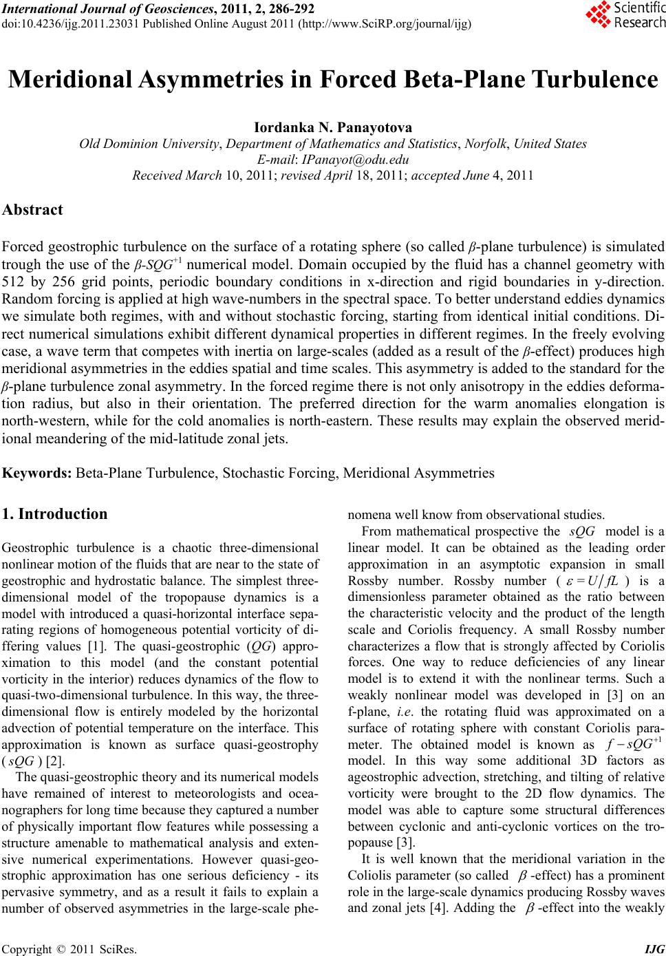
order to avoid its influence. The evolution of the freely
evolving 1
s
QG 

 surface potential temperature from
random inions shown in Figure 1. As it was
initially found in [5] inclusion of
itial condit

-effect in the higher-
order nonlinear dynamics added ave term that com-
petes with inertia on large-scales and produced high me-
ridional asymmetries in the eddies deformation radius.
This novel feature was added to the standard for the
a w

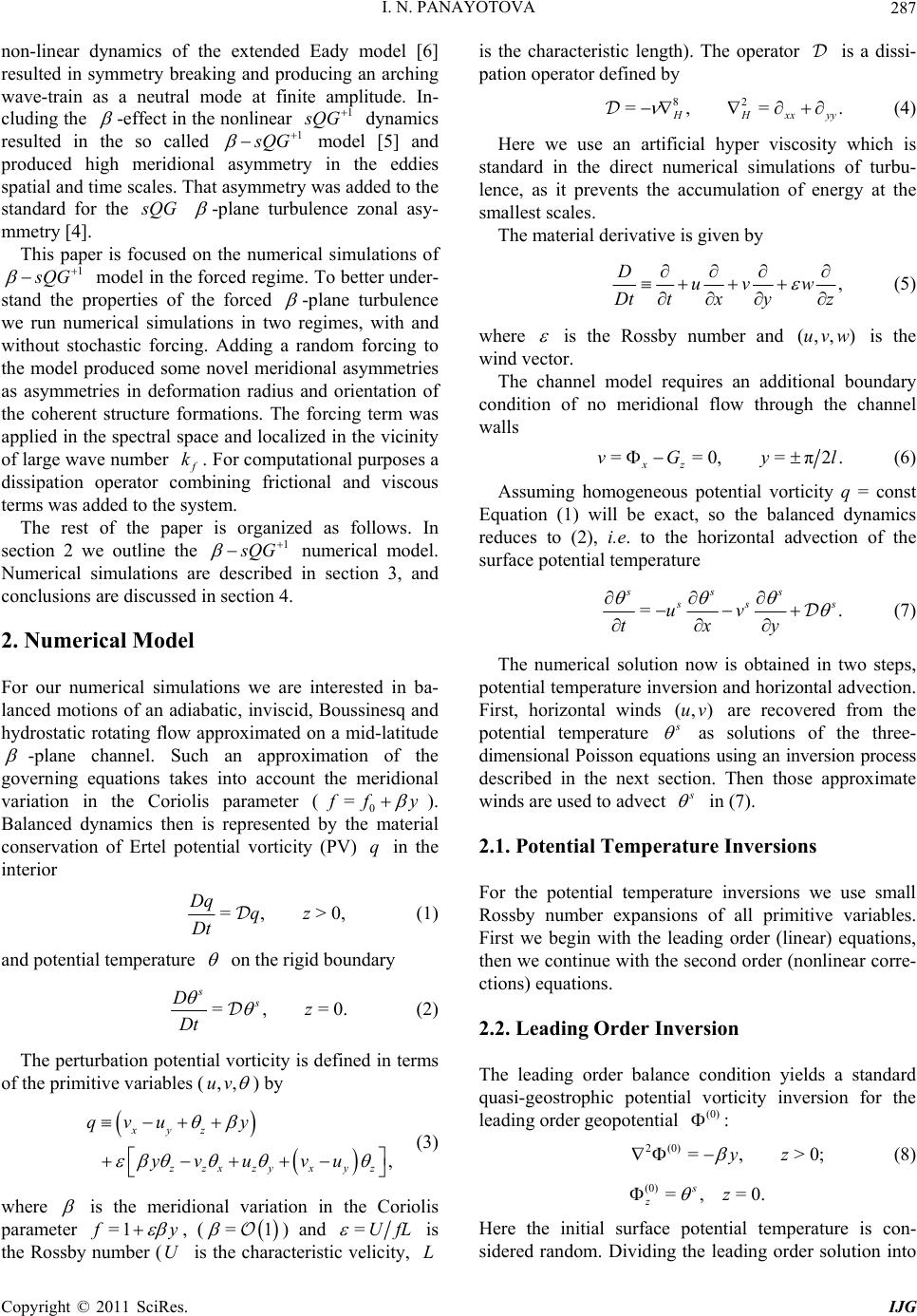
-plane turbulence zonal asymmetry, i.e. formed zonal
s. The zonal jet formation is shown in Figure 2.
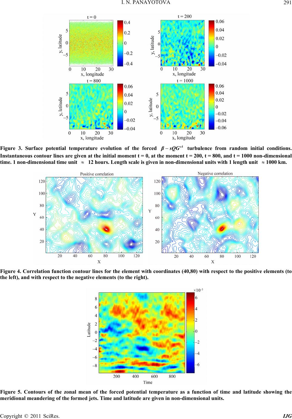
The evolution of the forced 1
jet
s
QG 

 turbulence
fo
ns of the formed
vo
(40,80) we ca-
lc
e of the zonal flow we calculated
tim
perty is in accordance with the well known from the ob-
rm random initial conditions is shgure 3. The
simulations in the forced regime exhibit not only ani-
sotropy in the eddies spatial and time scales, but also in
their orientation. In addition to the established wave-like
motion, after some time there is an evident tendency of
the flow to stretch vortices in preferred direction. As it
can be seen from the direct numerical simulations the
cold anomalies are always stretched in the north-
eastward direction, while the warm anomalies are stret-
ched in the north-westward direction.
However to catch exactly directio
own in Fi
rtices we used one point correlation method. The co-
rrelation function represents a statistical process, and as a
statistical quantity should be calculated over a long
interval of time. The correlation is large and positive if
the elements tend to be in a phase, i.e. positive picks tend
to occur together. The correlation is strongly negative, if
the elements are in the opposite phase, i.e. the peaks in
one occur when valleys are attained in the other. Finally,
the correlation function vanishes if the two variables are
90 degrees out-of-phase, i.e. one is passing through zero
at the peak or valley of the other.
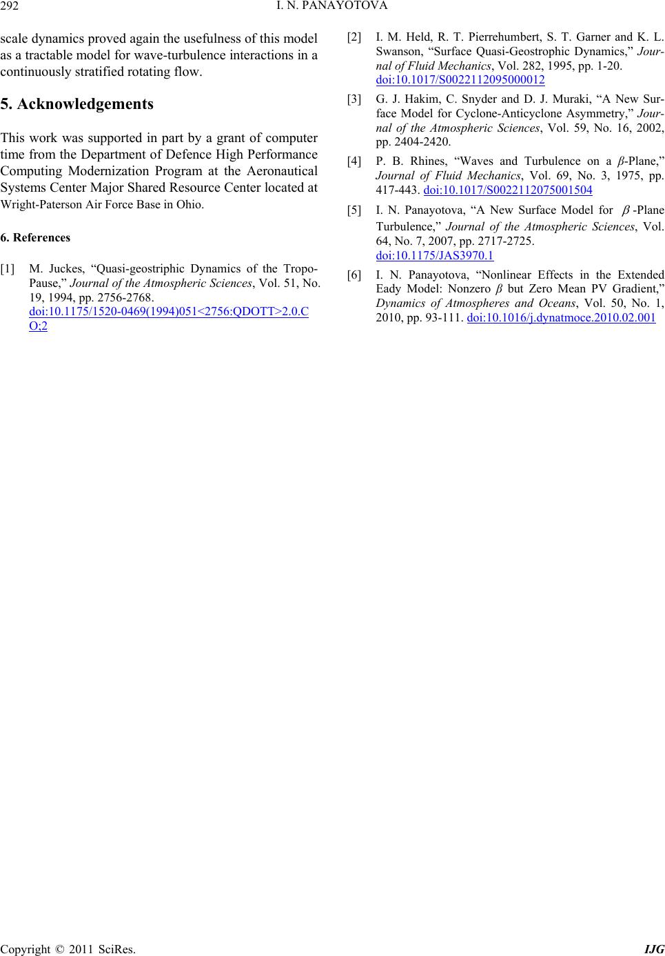
For a fixed element with coordinates
ulated its correlation with the others elements, and
correlation function contour lines are shown in Figure 4.
The left-hand side panel of Figure 4 shows positive
correlation of the reference point (40,80) with the other
elements, while the right-hand side panel represents the
negative correlation with the reference point. Those dire-
ctions coincide with the observed north-western elon-
gation of the worm anomalies and the north-eastern elon-
gation of the cold anomalies in the the potential tem-
perature evolution (3).
To see the persistenc
e sequence of the zonal mean of the potential tem-
perature at each latitude and the contour map is given in
Figure 5. This map illustrates that zonal jets are indeed
formed and in addition there is a meridional (northern/
southern) meandering of the formed jets. This novel pro-

I. N. PANAYOTOVA 290
Figure 1. Surface potential temperature evolution from random initial conditions of the freely evolving turbulence.
Instantaneous contour lines are given at the initial moment t = 0, at the moment t = 200, t = 800, and t = 1000dimensional
βsQG1
non-
km. time. 1 time unit  12 hours. Length scale is given in non-dimensional units with 1 length unit  1000
Figure 2. Contours of the zonal mean of the freely evolving potential temperature as a function of time and latitude showing
the jets formation. Time and latitude are given in non-dimensional units.
titudes.
usions
servational studies jet-meandering in the large-scale mid- forcing
la
4. Concl
Forced

-plane turbulence stabilized by large scale
ictionds to develop anisotropy and accumulate fr ten
n zenergy ional (or near zonal) modes. In this study we
showed something more, namely that forced

-plane
turbulence develops not only zonal, but also meridional
asymmetry. Direct numerical simulations presented here
illustrate the meridional meandering of the formed zonal
jets. The inclusion of the meridional variation in the
Coriolis parameter ( so called

-effect) into the weakly
nonlinear dynamics and the presence of some stochastic
orientation of the large-scale coherent structure
formations. A very intriguing novel feature of the forced
1
resulted in a theoretical model that captures both,
meridional asymmetries in the deformation radius and
s
QG 

 model was found, namely the warm ano-
malies are always elongated in the north-western dire-
ction while the cold anomalies are always oriented to the
north-east. The performed numerical simulations have
the combined presence of the shown that

-effect and
stochastic forcing have important influence on the large-
scale mid-latitude nonlinear atmospheric dynamics and
may explain the meridional meandering of the jet-
streams well known from the observationaltudies. The
fact that 1
s
s
QG 

 numerical model was able to cap-
ture those novel meridional asymmetries in the large-

I. N. PANAYOTOVA291
Figure 3. Surface potential temperature evolution of the forced βsQG 1

the moment
n in non-dime
turbulence from random initial conditions.
Instantaneous contour lines are given at the initial moment t = 0, at t = 200, t = 800, and t = 100 non-dimensional
time. 1 non-dimensional time unit 12 hours. Length scale is givensional units with 1 length unit 1000 km.
0
 
Figure 4. Correlation function contour lines for the element with coordinates (40,80) with respect to the positive elements (to
the left), and with respect to the negative elements (to the right).
Figure 5. Contours of the zonal mean of the forced potential temperature as a function of time and latitude showing the
meridional meandering of the formed jets. Time and latitude are given in non-dimensional units.

I. N. PANAYOTOVA 292
scale dynamics proved again the usefulness of this model
as a tractable model for wave-turbulence interactions in a
continuously stratified rotating flow.
5. Acknowledgements
This work was supported in part by a grant of computer
time from the Department of Defence High Performance
Computing Modernization Program at the Aeronautical
Systems Center Major Shared Resource Center located at
Wright-Paterson Air Force Base in Ohio.
6. References
[2] I. M. Held, R. T. Pierrehumbert, S. T. Garner and K. L.
Swanson, “Surface Quasi-Geostrophic Dynamics,” Jour-
nal of Fluid Mechanics, Vol. 282, 1995, pp. 1-20.
doi:10.1017/S0022112095000012
[3] G. J. Hakim, C. Snyder and D. J. Muraki, “A New Sur-
face Model for Cyclone-Anticyclone Asymmetry,” Jour-
nal of the Atmospheric Sciences, Vol. 59, No. 16, 2002,
pp. 2404-2420.
[4] P. B. Rhines, “Waves and Turbulence on a β-Plane,”
Journal of Fluid Mechanics, Vol. 69, No. 3, 1975, pp.
417-443. doi:10.1017/S0022112075001504
[5] I. N. Panayotova, “A New Surface Model for
[1] M. Juckes, “Quasi-geostriphic Dynamics of the Tropo-
Pause,” Journal of the Atmospheric Sciences, Vol. 51, No.
19, 1994, pp. 2756-2768.
doi:10.1175/1520-0469(1994)051<2756:QDOTT>2.0.C
O;2

-Plane
Turbulence,” Journal of the Atmospheric Sciences, Vol.
64, No. 7, 2007, pp. 2717-2725.
doi:10.1175/JAS3970.1
[6] I. N. Panayotova, “Nonlinear Effects in the Extended
Eady Model: Nonzero β but Zero Mean PV Gradient,”
Dynamics of Atmospheres and Oceans, Vol. 50, No. 1,
2010, pp. 93-111. doi:10.1016/j.dynatmoce.2010.02.001