Coupled Effects of Energy Dissipation and TravellingVelocity in the Run-Out Simulation of High-SpeedGranular

doi:10.4236/ijg.2011.23030

Paper Menu >>

Journal Menu >>

International Journal of Geosciences, 2011, 2, 274-285

doi:10.4236/ijg.2011.23030 Published Online August 2011 (http://www.SciRP.org/journal/ijg)

Coupled Effects of Energy Dissipation and Travelling

Velocity in the Run-Out Simulation of High-Speed

Granular Masses

Francesco Federico1, Giuseppe Favata

1University of Rome “Tor Vergata”, Rome, Italy

E-mail: fdrfnc@gmail.com

Received February 1, 2011; revised April 5, 2011; accepted June 2, 2011

Abstract

The run-out of high speed granular masses or avalanches along mountain streams, till their arrest, is analyti-

cally modeled. The power balance of a sliding granular mass along two planar sliding surfaces is written by

taking into account the mass volume, the slopes of the surfaces, the fluid pressure and the energy dissipation.

Dissipation is due to collisions and displacements, both localized within a layer at the base of the mass. The

run-out, the transition from the first to the second sliding surface and the final run-up of the mass are de-

scribed by Ordinary Differential Equations (ODEs), solved in closed form (particular cases) or by means of

numerical procedures (general case). The proposed solutions allow to predict the run-up length and the speed

evolution of the sliding mass as a function of the involved geometrical, physical and mechanical parameters

as well as of the simplified rheological laws assumed to express the energy dissipation effects. The corre-

sponding solutions obtained according to the Mohr-Coulomb or Voellmy resistance laws onto the sliding

surfaces are recovered as particular cases. The run-out length of a documented case is finally back analysed

through the proposed model.

Keywords: Sliding Granular Mass, Granular Temperature, Shear Layer, Excess Interstitial Pressure

1. Introduction

Great attention receives in scientific community the study

of kinematic mechanisms of the flow of viscous fluid [1]

or the chaotic movement of granular masses [2], because

their destroying effects, often related to increasing an-

thropization of piedmont areas. It is necessary to identify

hazardous areas for the propagation of high-speed mov-

ing masses. To this purpose, reliable criteria must be for-

mulated and applied.

Interstitial pressures at the base of the mass can vary

from null or hydrostatic value to high values, due to

possible water pressure excess, related to very rapid

changes of pore volumes, often localized along a thin

layer in proximity of the sliding surface [3].

Several models assume the validity of the Mohr-Cou-

lomb (M-C) shear resistance criterion [4] along the slid-

ing surface of the high-rate moving mass. To match ex-

perimental observations of the run-out length with theo-

retical results, small shear resistance angles must be

assumed. The M-C law usually describes limit equili-

brium (static) or simple sliding of blocks along rough

surfaces (dynamic condition). More complex resistance

laws should be taken into account [5] to describe the

rapid sliding of granular masses because high speed

relative motion and collisions between solid grains take

place within a basal shear layer, causing a fluidification

effect coupled with energy dissipations [6]. Therefore, it

is not conceptually justifiable the reduction of the shear

resistance angle, due to the high mobility of the grains [7]

if the corresponding energy dissipation is not taken into

account. Moreover, in situ observations show that the

run-out length strongly depends on the mobilized volume

of the mass [8-11].

In the paper, the rapid sliding of a granular mass along

two planar surfaces is analytically modelled by account-

ing for the effects of grain collisions.

In section 2 the main features of the model and the

assumed simplifying hypotheses are introduced; the go-

verning equations are formulated (section 3), by intro-

ducing the parameters which take into account the gra-

nular temperature and the collisional dissipated energy.

F. FEDERICO ET AL.275

Closed form or numerical solutions of the ODEs are then

obtained (section 4). After an estimate of the model para-

meters, in section 5 some parametric results of run-out

length are represented and compared to solutions ob-

tained according to the M-C or Voellmy (V) resistance

criteria along the base of the sliding mass. The schematic

back analysis of a case is carried out through the model

in section 6. Some concluding remarks close the paper.

2. Analytical Model

2.1. Basic Assumptions

Three phases roughly characterize rapid landslides mo-

tion, after their detachment (avalanches) or trigger (de-

bris flow): 1) the mass runs along the first sliding surface

(s.s.) (run-out), 2) the initial portion of the mass slides

along the counterslope s.s. while the remaining portion

still moves along the first one, 3) the whole mass runs up

along the counterslope s.s., till its stop (Figure 1).

Moreover:

 Planar sliding surfaces are assumed (Figure 1): the

slope angles of the first and second s.s. are



> 0 and



 0, respectively. The run-out length along the first

surface is L;

Figure 1. (a) Phases of rapid landslides or avalanches mo-

tion: I - detachment and initial conditions; II - run-out; III -

transition of the moving mass from the first to the second

inclined planar surface; IV - run-up; V – final position; (b)

shear layer in proximity of the basal sliding surface;, fluc-

tuations of particles velocity around their average value,

occur; (c) problem setting for computations; (d) transition

from the first to the second sliding plane.

 the sliding granular mass is schematized as a paral-

lelepiped (length l, height H and depth D) whose

geometry doesn’t vary; erosion or deposition proc-

esses are not considered;

 a “shear layer” at the base of the mass takes place

during the rapid sliding. This small thickened layer

(compared to H) is composed by particles that move

at high velocity and collide each with others. Colli-

sions induce appreciable fluctuations of their veloci-

ties (granular temperature);

 the energy dissipation due to the mass straining cou-

pled with the mass displacements, is neglected.

2.2. Governing Equations

The power balance of the sliding mass holds:

ddd d0

dd dd

pcna na

EEE E

tt tt



 

(1)

Ep being the potential energy, Ec the kinetic energy of the

sliding mass. The dissipated energy (Ena), not more avai-

lable for the motion, is schematically splitted in two

components: Ena1, lost due to the (Coulomb’s) friction

along the sliding surface; Ena2, transferred from the block

to the basal “shear layer” [2,7,12]. The (1) is in the fol-

lowing rewritten for each phase of the motion.

2.3. Transfer and Dissipation of Energy

Ena1 is a function of the weight W of the sliding mass,

the resultant U of the interstitial fluid pressures, the shear

resistance angle



b at the base of the block, reduced with

respect to the shear resistance angle



’ of the involved

material, due to the peculiar physical conditions (high

speed, collisions) along the s.s., the path x.

The energy Ena2 transferred to the “shear layer” [2,7,

12], is lost by the granular mass during its running along

the first s.s.;, Ena2 may be partially recovered by the mass

and correspondingly lost by the “shear layer”, along the

run-up (counterslope). The analytical expression of Ena2

is not a priori known: it is hypothesized its dependence

upon the rate v of the granular mass. As stated by [6], the

maximum value of the function dEna2/dt is obtained if the

rate )(

1txv 



attains a constant value, whatever be its

value. Therefore, dEna2/dt has been defined as follows:



max

na na











(2)

the adimensional function depending on v.







1











, the energy is not transferred from the

mass to the shear layer (granular temperature) or vice-

versa; the limit case









 implies that the energy

transfer is maximized, being v = const.

F. FEDERICO ET AL.

276

2.4. Effects of Interstitial Pressures

The interstitial pressurew(x) at the base of the mass

affects the run-out length; w(x) simply assumes the

constant value (nil value as limit case) through the

relation: ww (Figure 1),



w being the spe-

cific weight of the water; d = 0 if the whole mass is

saturated; d = H if the mass is dry; wmay exceed the

hydrostatic value due to the mechanical effects associ-

ated with the rapid change of intergranular volumes of

the voids and the corresponding growth of interstitial

water pressures excess [3,6]. To simulate this effect, d <

0 values must be assigned. The length d thus lies in the

range:



Hd







min max

ddd (3)

If the sliding granular mass always transmits positive

normal stresses to the s.s., through the shear layer, the

minimum value min can be deduced by imposing the

equilibrium along the direction orthogonal to the sliding

plane:

min mincos1 ;cos1













  





















(4)



t being the unit weight of the sliding mass and dmin a

negative real number.

2.5. Sliding along the First Slope

The potential energy

E in the power balance (1) is

rewritten in function of the abscissa x1 (Figure 1) as fol-

lows:





sin

Emghx



 (5)

h0 being the initial elevation of the centre of mass with

respect to a reference plane; g the gravity acceleration

and m the mass of the sliding granular body.

The dissipated energy





11na

is then rewritten as

follows:

 



11 0

costan d

costan

na b

ExW Us

WUx





 (6)

U < Wcos



being the global force associated with the

pressure wat the base of the mass, W the mass weight

and



b the reduced shear resistance angle at the base of

the mass.

The dissipated energy Ena2 (2) depends upon the rate v

of the granular mass.

According to (5), (6), the equation (1) is rewritten as:

 



sin 2

+costand

mgx tmdtE

WUxt











(7)

The maximum value for dEna2/dt is gained if





vxt assumes a constant value [6]. It may be writ-

ten:



max

dsincos tan

na b

EWWUx













(8)

Recalling the (2), dEna2/dt becomes:

 

dsincos tan

na b

EvWW Uxt









 (9)

the function











 being previously introduced.

By replacing the (9) in (7), it is obtained:







 

sincostan 1

dx t

vxt



 





 













(10)

The ratio U/W is rewritten as:





HdlD

WHlD

















(11)

So, the Equation (11) becomes:









tan

tantan11( )

cos

dx t

vxt





 























(12)

Let be



,, 11

cos

RR dH





















(13)

The derivative of equation (12) gets:











1cos tantan1

tg Rv



 















(14)

According to the assumed hypotheses, the time deriva-

tive of the energy component Ena2, for unit mass, is:



dcos tantan

na b



 

 (15)

Through the (15), the discriminant value



* for which

dEna2/dt = 0 may be determined, by solving the equation:







cos tantan0



 



 (16)

If the slope angle





*, dEna2/dt < 0: the sliding

mass receives energy from the shear layer. If





dEna2/dt > 0: the sliding mass provides energy to the

shear layer.

Being interesting only the conditions and

cos 0









*0v





, according to the (13), the (16) becomes:

F. FEDERICO ET AL.277

tan1tan 0

cos b







 







(17)

Through the (17),



* is obtained:

2424

tan

arccos cottan1(tan )

(tan )(tan )(tan )

1(tan )

bb b





































(18)





wt dH







(19)

In the simple case d = H (no interstitial fluid pressure),

it results



= 0 and the equation (18) gets



* =



The sign of the derivative dEna2/dt depends on the sign

of the expression



tantan b





, the other terms

being positive. This sign is positive along the first planar

s.s. (otherwise, the motion cannot take place), while is

negative along the second s.s., because we must replace



> 0 with





* (reduced slope) or



≤ 0 (counter-

slope).

2.6. Sliding along the Counterslope Surface

The motion law along the counterslope s.s. is obtained by

substituting in the (14) the angle



> 0 with



≤ 0; cor-

respondingly, the function





(v) must be replaced by





(v):







2cos tantan1

tg Rv



 







 (20)

where:

cos









 









(21)

The ODE (20) must be solved taking into account the

following initial conditions:

 

00; 0

xv



v0 being the velocity of the mass after the full transition

from the first to the second sliding planar surface.

2.7. Transition from the First to the Second Slope

By neglecting the additional lost of energy coupled with

peculiar strains associated with the slope change of the

s.s., the ODE expressing the motion during the transition

phase may be approximated through the linear combina-

tion of (14) and (20):









 





12 1

12 2

cos tantan1

cos(tantan)10

xt gRv lt





 

 

















(22)

l1(t) being the length of the portion of the granular

mass resting on the first surface and l2(t) = x12(t) the

length of the remaining part running up along the second

plane (run-up). So, l1(t) + l2(t) = l, neglecting second or-

der geometrical aspects and accounting for the consider-

able length of the sliding granular mass (Figure 1(d)).

After some algebra, Eqution (22) can be written as:



 



 

12 12

cos tantan1

tRvl

gRvxt





 

 











 xt



(23)

The second term figuring in the expressions R and R

represents the contribution due to interstitial pressures; it

is always positive because d



H. By decreasing d (the

free surface moves towards the top of the mass) R and

R decrease; the terms





tantan b





 and





tantan b





 consequently increase. So, all other

factors assuming constant values, the acceleration will be

as greater as smaller is d.

2.8. Acceleration and limit rate

Referring to the acceleration along each sliding surface,

equations (14) and (20) can be rewritten as follows:













cos tantan1

tg Rv











 (24)

where:

cos









 









(25)

0 for 0

0 for















 (26)

The term





cos 1rv gv























01v





is always posi-

tive along both sliding surfaces (). If the

increase of the function





(v) with the rate v of the mass

is assumed, the function r(v) will decrease if v increases.

Equation (24) can be thus rewritten as:













tantan b

xt rvR







 (27)

Coefficient 1R





is equal to one if the interstitial

pressures are equal to zero. Along the first surface,

tan tanR







, otherwise, the initial conditions









00,x00x



 would not allow the motion begin-

ning; thus, the acceleration will be positive, the sliding

rate will increase, r(v) will decrease and, consequently, a

decrease of acceleration, always positive, will occur

along the path. The acceleration will vanish if the rate

approaches its limit value, for which , or



lim 0rv





lim 1v





.

F. FEDERICO ET AL.

278

Along the second inclined plane, tantan0





:

therefore, the acceleration now assumes negative values,

the sliding rate will decrease, r(v) will increase and,

consequently, the absolute value of acceleration (which

is, however, negative) will increase.

3. Mathematical Model

3.1. The



(v) Function

The function





(v) governs both transfer and dissipation

of energy taking place near the sliding surfaces, due to

multiple collisions between particles, as well as rotations

of each particle around an axis [6]. The function







0,1v





 has been analytically represented through

a second order, rate increasing polynomial function:







 v



(28)

0 being an adimensional constant;





and





are con-

stants whose dimensions are the inverse of velocity and

the inverse of square velocity, respectively (







If , it is obtained . The limit

value of the rate corresponding to of the slid-

ing mass may be obtained by imposing:



lim 1v









10xt





10xt



0lim lim

1vv



 

 

(29)

The (29) gets:



lim







 



 

 (30)

The negative solution of (30) is not significant.

Coefficients







and





cannot assume arbitrary

values; they must respect the conditions deriving from

the inequalities as well as from the definition domains of

the integration constants (see sections 3.3 and 3.4), re-

ported in Table 1.

3.2. Equations of Motion

After substitution of (28) in (14), (20) and (22), the equa-

tions of motion, are written as follows:

Table 1. Imposed conditions on the coefficients of the model,

(v) being expressed by (28).

Condition









41 0



 









 









111

0xtABxtCx t



 

  (31)





222

0xt DExt Fxt





  (32)

 



  

1212 1212

12 1212 1212

12 1212120

tABxt Cxtxt

BCD

tx txtxx t

lll

xtxt xtxt

  











(33)

where



 

cos tantan1

Ag R









 (34a)





costantan b

Bg R







 (34b)





costantan b

Cg R





 

 (34c)



 

cos tantan1

DgR









 (34d)





costantan b

Eg R





 

 (34e)





costantan b

Fg R





 

 (34f)

3.3. Analytical Solution: Sliding along the First

Slope

The integration of Equation (31) gets:







tanh2

xtBCCB AC

BACCCt































(35)

 





112

2lncosh2

xtBC CtCC

BACCCt





































(36)

The unknown constants C1 and C2 are determined

through the initial conditions:





00, 00xx





122

2arctanh

CBAC BAC











(37a)

222

arctanh

11 4

ln2

CCBACBAC

BAC

CAC





















(37b)

3.4. Analytical Solution: Sliding along the

Second Slope

The analytical integration of (32) (counterslope) gets:

F. FEDERICO ET AL.279







tanh2

xtEFFEDF

EDFCFt

 



























(38)







2lncosh 2

xtEC FtFC

EDFCFt









































(39)

By imposing the conditions:

 

00, 0

xv



the unknown constants are determined:

322

2arctanh

CEDF EDF























(40a)



422

arctanh

11 4

ln242

Fv E

CFEDFe DF

EDF

FEDFFvE





















 









(40b)

3.5. Transition from the First to the Second

Slope

The integration of (33) is carried out by means of a nu-

merical procedure, by assigning initial conditions:

 

1212 1

00, 0

xv



v1f being the rate of the sliding granular mass at the end

of the first inclined planar s.s. To this aim, the fourth

order Runge-Kutta method with adaptive step size has

been implemented in MathCad.

It is worth observing that the proposed analytical solu-

tions have been found referring to the trinomial formula



(v) (28). If



(v) is simply expressed by assuming



(v)

= 0 or



(v) = 0 or both, it is possible to express the ana-

lytical solution in closed form, also for the transition

from the first towards the second s.s.

4. Characterization of the



(v) function

4.1. Premise

The limits of the function





(v) (Eqution (20)) are the

same as those assumed for the function





(v). Part of the

energy is given back to the sliding mass by the shear

layer, whose granular temperature gradually decreases,

due to the corresponding decrease of the average run-up

rate. If the inequalities are taken into

account, the maximum negative variation of lost energy,

as well as the maximum variation of energy recovered by

the sliding granular mass, cannot exceed the maximum

value corresponding to the limit case v = cost. The time

variation of energy lost due to granular temperature then

assumes negative values along the second sliding surface;

thus, the granular mass recovers energy by the shear

layer. The function





(v) modulates the part of energy

unavailable for the motion; it incorporates the effects due

to granular temperature and collisional dissipations along

the first inclined plane;





(v), the part of energy given

back to the sliding granular mass, net collisional dissipa-

tions; then,





(v) cannot be equal to





(v): the inequality







1













v must always hold.

4.2. Coefficients

To estimate the parameters











(function





(v)), it

is first analyzed the simpler case 0





.





is linearly

related to the sliding rate and it is roughly correlated to

the macro-viscous regime [14,15] that takes place only

for small velocities of the granular mass; for a long and

rapid sliding path, it does not seem prevalent.

Attention is so focused to





, by assuming that



0 as-

sumes the same value along both the sliding surfaces.





cannot assume the same value along the two s.s.

Along the first surface (









modulates the power

subtracted to the granular mass, not available for the mo-

tion. A part, here defined



, is stored as power related to

granular temperature; the remaining part,



, is lost due to

the collisions associated to the granular temperature.

Therefore,





analytically expresses the sum of the pow-

ers related both to the granular temperature and colli-

sional dissipation:



















(41)

Along the counterslope plane (





), the “stored”

power



is partly given back to the sliding mass (







and partly dissipated through collisions. Therefore,





represents the power given back to the granular mass; it

must express the difference between the power previ-

ously “stored” (



) and the power again dissipated (













 







(42)





represents the ratio between the powers (Ecoll) lost

due to collisions and (Egt) stored through the granular

temperature:

coll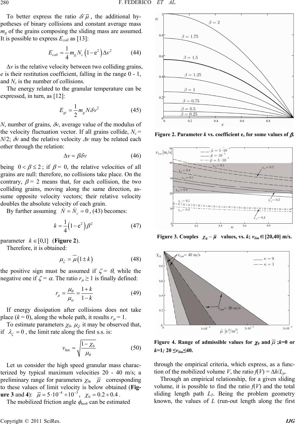









 (43)

F. FEDERICO ET AL.

280

To better express the ratio





, the additional hy-

nstant average mass potheses of binary collisions and co

mg of the grains composing the sliding mass are assumed.

It 13]: is possible to express Ecoll

as [



11e

collg c

EmNv (44)

between two colliding v is the relative velocitygrains,

e is their restitution coefficient, falling in the

and Nc is the number of collisions.

range 0 - 1,

The energy related to the granular temperature can be

expressed, in turn, as [12]:

gt g

EmNv



 (45)

N, number of grains,



v, average value of the modulus of

the velocity fluctuation vector. If all gr

N/2;



v and the relative velocity



v may be related each

ains collide, Nc =

other through the relation:





 (46)

being 02



; if



= 0, the relative velocities of all

grains are null: therefore, no collisi

contrary,



= 2 means that, for ea

g grains

ons take place. On the

ch collision, the two

collidin, moving along the same direction, as-

sume opposite velocity vectors; their relative velocity

doubles the absolute velocity of each grain.

By further assuming 0

NN

 , (43) becomes:



11e



 (47)

parameter (

Figure 2).

Theref is obtained:

]1,0[k

ore, it





k (48)

thssumed if





, while the

negative one if





. The ratio r



≥ 1







e positive sign must be a

is finally defined:













 (49)

If energy dissipation after collisions doe

place (k = 0), along the whole path, it

To estimate parameters







, it may be observed that,

s not take

results r



= 1.





, the limit rate along the first s.s. is:

lim









 (50)

Let us consider the high speed granula

terized by typical maximum velocitie

preliminary range for parameters



r mass charac-

s 20 - 40 m/s; a



Figure 2. Parameter k vs. coefficient e, for some values of





Figure 3. Couples values, vs. k; vlim∈[20,40] m/s.



;Figure 4. Range of admissible values for



0 andk=0 or

k=1; 20 ≤vlim≤40.

zed volume V, the ratio f(V) = h/Lp.

Through an empirical relationship, for a given sliding

through the empirical criteria, which express, as a func-

tion of the mobili

corresponding

to these values of limit velocity is below obtained (Fig-

ure 3 and 4): 43

510 10





 , 00.20.4



.

The mobilized friction angle



mob cae estimated n b

volume, it is possible to find the ratio f(V) and the total

sliding length path LT. Being the problem geomet

own, the values of L (run-out length along the first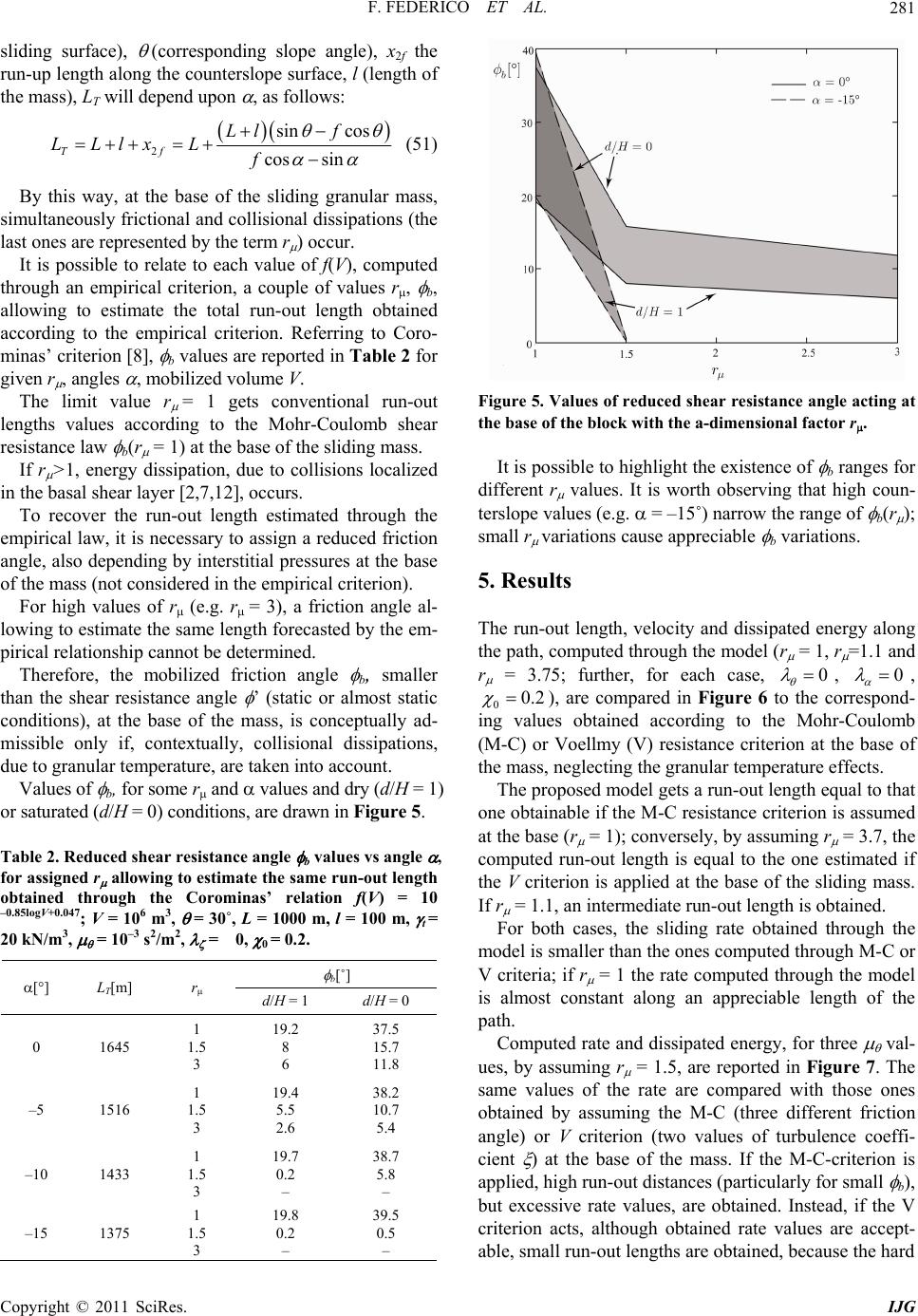

F. FEDERICO ET AL.281

sliding surface),



(corresponding slope angle), x2f the

run-up length along the counterslope surface, l (length of

the mass), LT will depend upon



, as follows:

 

sin cos

cos sin

Ll f

LLlx Lf







  (51)

By this way, at the base of the sliding granular m

simultaneously frictional and collisional dissipation

last ones are represented by the term r



) occur.

obtained

sliding mass.

sures at the base

ncepally ad-

ob ined through the Corominas’ relation f(V) = 10

ass,

s (the

It is possible to relate to each value of f(V), computed

through an empirical criterion, a couple of values r,



allowing to estimate the total run-out length

cording to the empirical criterion. Referring to Coro-

minas’ criterion [8],



b values are reported in Table 2 for

given r



, angles



, mobilized volume V.

The limit value r



= 1 gets conventional run-out

lengths values according to the Mohr-Coulomb shear

resistance law



b(r



= 1) at the base of the

If r



>1, energy dissipation, due to collisions localized

in the basal shear layer [2,7,12], occurs.

To recover the run-out length estimated through the

pirical law, it is necessary to assign a reduced friction

angle, also depending by interstitial pres

the mass (not considered in the empirical criterion).

For high values of r (e.g. r= 3), a friction angle al-

lowing to estimate the same length forecasted by the em-

pirical relationship cannot be determined.

Therefore, the mobilized friction angle



b, smaller

than the shear resistance angle



’ (static or almost static

conditions), at the base of the mass, is cotu

issible only if, contextually, collisional dissipations,

due to granular temperature, are taken into account.

Values of



b, for some r and  values and dry (d/H = 1)

or saturated (d/H = 0) conditions, are drawn in Figure 5.

ble 2. Reduced shear resistance angle



b values vs angle



for assigned r



allowing to estimate the same run-out length

–0.85logV+0.047; V = 106 m3,



= 30˚, L = 1000 m, l = 100 m,



t =

20 kN/m3,





= 10–3 s2/m2,





= 0,



0 = 0.2.



b[˚]

[°]LT[m] r d/H = 1 d/H = 0

0 1645

Figure 5. Values of reduced shear resistance angle acting at

the base of the block with the a-dimensional factor r.

It is possible to highlight the existence of



b ranges for

different r



values. It is worth observing that high cou

= 3.75; further, for each case,

terslope values (e.g. = –15˚) narrow the range of



b(r



);

small r



variations cause appreciable



b variations.

Results

The run-out length, velocity and dissipated energy along

the path, computed through the model (r



= 1, r



=1 and







, 0







00.2





), ar

g values obtained

e compared in Figure 6to the correspond-

according to thehr-C

th e tha

obta

ss.

or criterion (two values of turbulence coeffi-

Moinoulomb

(M-C) or Voellmy (V) resistance criterion at the base of

the mass, neglecting the granular temperature effects.

The proposed model gets a run-out lengqual tot

one inable if the M-C resistance criterion is assumed

at the base (r



= 1); conversely, by assuming r



= 3.7, the

computed run-out length is equal to the one estimated if

the V criterion is applied at the base of the sliding ma



= 1.1, an intermediate run-out length is obtained.

For both cases, the sliding rate obtained through the

model is smaller than the ones computed through M-C or

V criteria; if r



= 1 the rate computed through the model

is almost constant along an appreciable length of the

path.

1 19.2

37.5

15.7 1.5

3 6 11.8

–5 1516

1.5

19.4

5.5

2.6

38.2

10.7

5.4

–10 1433

1.5

19.7

0.2

–

38.7

5.8

–

Computed rate and dissipated energy, for three





val-

ues, by assuming r



= 1.5, are reported in Figure 7. The

same values of the rate are compared with those ones

obtained by assuming the M-C (three different friction

angle) V

ent



) at the base of the mass. If the M-C-criterion is

applied, high run-out distances (particularly for small



b),

but excessive rate values, are obtained. Instead, if the V

criterion acts, although obtained rate values are accept-

able, small run-out lengths are obtained, because the hard

–15 1375

1.5

19.8

0.2

–

39.5

0.5

–

F. FEDERICO ET AL.

282

Figure 6. Velocity (v) along the path and energy dissipation

(E) for three values of r



; L = 1000m, l = 100 m, H = 5 m, d =

0 m,



b = 10˚,  = 30˚,



= 0˚,



t = 20 kN/m3. For Voellmy

criterion,



= 1000 m/s2.

deceleration of the mass at the slope change. Computed

. Back analysis

l model [16,17]

ble and are not directly

pplicable to estimate the above defined parameters. By

ese limits, the back analysis of the

n-out length measured for the Frank slide (Canada,

water saturated mass has been

run-out lengths LT considerably vary with

counterslope, Figure 8 and ratio d/H (interstitial

pressures at the base, Figure 9).

Only a partial assessment of the theoretica

is possible, since direct field observations of landslides

and avalanches are rarely availa

taking into account th

1903) is carried out.

The Frank slide occurred on the morning April 29,

1903, killing about 70 people. The estimated mobilized

volume was about 30 × 106 m

3. The slope of the first

sliding surface is about 30˚, while for the counterslope is

about –2.2˚. The profile along the run-out path is repre-

sented in Figure 10. A

Figure 7. Velocity (v) along the path and energy dissipation

(E); L = 1000 m, l = 100 m, H = 5 m, d = 0 m,



= 30˚,



= 0˚,



t = 20 kN/m3. For Voellmy criterion, it is assigned



b = 10˚.

Figure 8. Total run-out length (LT) vs counterslope angle ;

L = 1000 m, l = 100 m, H = 5 m,  = 30˚, t = 20 kN/m3, r=

1.5,





0,



b = 10˚,





=5 · 10–4.

F. FEDERICO ET AL.

283

Figure 9. Total run-out length (LT) vs. ratio d/H; L = 1000 m, l = 100 m, H = 5 m,  = 30˚,



t = 20 kN/m3, r



= 1.5,





0,



b =

10˚,



= 0˚





=5 · 10–4.

Figure 10. Frank slide: profile along e run-out path (modified from [17]).

A basal shear resistance angle equal to 16° has been

assigned, according to [16]. The parameters assigned to

fit the measured run-out length LT = 2800 m are:









= 5·10–5 s/m,



0 = 0.1,





= 3·10–4 s2/m2.

The rate along the path is reported in Figure 11, for

three r values. An acceptable agreement between meas-

ured and computed run-out lengths is achieved for r =

1.25.

The max rate of the sliding mass is 50 m/s, almost in-

dependently from the r values.

7. Concluding remarks

The motion of a granu

odeled accounting for granular temperature effects [6].

g to experimental observations and theoreti-

related storage

of kinetic energy, due to fluctuations of grains velocity,

occur within this s.l.

The energy transferred by the s.l. (granular-inertial re-

gime) to the sliding mass and viceversa, following a

suggestion by [6], has been modeled by introducing a

positive adimensional rate dependent function





(v) in

the power balance of the sliding mass.

By this way, the governing equations of the motion

have been written with reference to the sliding along: 1)

the first s.s.; 2) the progression from the first (



>0) to

the second s.s. (



<0); 3) the run-up along the second s.s.

The assumption of a reduced shear resistance (mobilized

angle



b <



’) in Corominas’ empirical criterion is con-

dissipation related to

assumed.

lar mass along two planar s.s. is ceptually justified only if the energy

grains collisions, localized in the shear layer, is consid-

med; a possible range of



b values has been evaluated.

The “transfer” function





(v) plays a role on the ef-

fects of energy dissipation and on the kinematic of the

mass.

Accordin

l considerations, it is assumed that, during the rapid

motion, a shear layer (s.l.) at the base of the sliding mass

takes place [2,7,12]. Energy dissipation due to both fric-

tional and collisional phenomena [13] andMoreover, along the first s.s., acceleration is smaller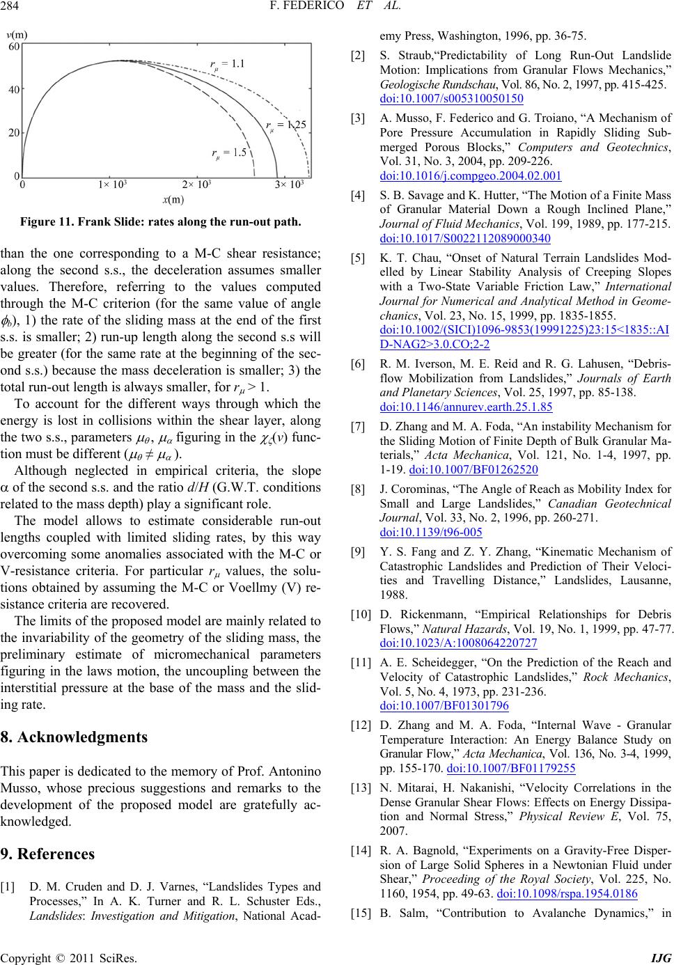

F. FEDERICO ET AL.

284

Figure 11. Frank Slide: rates along the run-out path.

coupled with limited sliding rates, by this

V-resistance criteria. For particular r



values, the solu-

tions obtained by assuming the M-C or Voellmy (V) re-

sistance criteria are recovered.

The limits of the proposed model are mainly related to

the invariability of the geometry of the sliding mass, the

preliminary estimate of micromechanical param

figuring in the laws motion, the uncoupling between

interstitial pressure at the base of the mass and the slid-

ing rate.

8. Acknowledgments

his paper is dedicated to the memory of Prof. Antonino

Landslides: Investigation and Mitigation, National A

[2]

an the one corresponding to a M-C shear resistance;

along the second s.s., the deceleration assumes smaller

values. Therefore, referring to the values computed

through the M-C criterion (for the same value of angle



b), 1) the rate of the sliding mass at the end of he first

s.s. is smaller; 2) run-up length along the second s.s will

be greater (for the same rate at the beginning of the sec-

ond s.s.) because the mass deceleration is smaller; 3) the

total run-out length is always smaller, for r



> 1.

To account for the different ways through which the

energy is lost in collisions within the shear layer, along

the two s.s., parameters









figuring in the





(v) func-

tion must be different (





≠





Although neglected in empirical criteria, the slope

of the second s.s. and the ratio d/H (G.W.T. conditio

lated to the mass depth) play a significant role.

The model allows to estimate considerable run-out

lengths way

ercoming some anomalies associated with the M-C or

eters

the

Musso, whose precious suggestions and remarks to the

development of the proposed model are gratefully ac-

knowledged.

. References

[1] D. M. Cruden and D. J. Varnes, “Landslides Types and

Processes,” In A. K. Turner and R. L. Schuster Eds.,

emy Press, Washington, 1996, pp. 36-75.

ca d-

S. Straub,“Predictability of Long Run-Out Landslide

Motion: Implications from Granular Flows Mechanics,”

Geologische Rundschau, Vol. 86, No. 2, 1997, pp. 415-425.

doi:10.1007/s005310050150

[3] A. Musso, F. Federico and G. Troiano, “A Mechanism of

Pore Pressure Accumulation in Rapidly Sliding Sub-

merged Porous Blocks,” Computers and Geotechnics,

Vol. 31, No. 3, 2004, pp. 209-226.

doi:10.1016/j.compgeo.2004.02.001

[4] S. B. Savage and K. Hutter, “The Motion of a Finite Mass

of Granular Material Down a Rough Inclined Plane,”

Journal of Fluid Mechanics, Vol. 199, 1989, pp. 177-215.

doi:10.1017/S0022112089000340

[5] K. T. Chau, “Onset of Natural Terrain Landslides Mod-

elled by Linear Stability Analysis of Creeping Slopes

with a Two-State Variable Friction Law,” International

Journal for Numerical and Analytical Method in Geome-

chanics, Vol. 23, No. 15, 1999, pp. 1835-1855.

doi:10.1002/(SICI)1096-9853(19991225)23:15<1835::AI

D-NAG2>3.0.CO;2-2

6] R. M[. Iverson, M. E. Reid and R. G. Lahusen, “Debris-

Landslides,” Journals of Earth

ol. 25, 1997, pp. 85-138.

doi:10.1146/annurev.earth.25.1.85

flow Mobilization from

and Planetary Sciences, V

10.1007/BF01262520

[7] D. Zhang and M. A. Foda, “An instability Mechanism for

the Sliding Motion of Finite Depth of Bulk Granular Ma-

terials,” Acta Mechanica, Vol. 121, No. 1-4, 1997, pp.

1-19. doi:

]J. Corominas, “The Angle of Reach as Mobility Index for

rge Landslides,” Canadian Geotechnical

, No. 2, 1996, pp. 260-271.

Small and La

Journal, Vol. 33

doi:10.1139/t96-005

[9] Y. S. Fang and Z. Y. Zhang, “Kinematic Mechanism of

Catastrophic Landslides and Prediction of Their Veloci-

ties and Travelling Distance,” Landslides, Lausanne,

1988.

[10] D. Rickenmann, “Empirical Relationships for Debris

Flows,” Natural Hazards, Vol. 19, No. 1, 1999, pp. 47-77.

doi:10.1023/A:100806422072

[11] A. E. Scheidegger, “On the Prediction of the Reach and

Velocity of Catastrophic Landslides,” Rock Mechanics,

Vol. 5, No. 4, 1973, pp. 231-236.

doi:10.1007/BF01301796

[12] D. Zhang and M. A. Foda, “Internal Wave - Granular

Temperature Interaction: An Energy Balance Study on

Granular Flow,” Acta Mechanica, Vol. 136, No. 3-4, 1999,

pp. 155-170. doi:10.1007/BF01179255

[13] N. Mitarai, H. Nakanishi, “Velocity Correlations in the

doi:10.1098/rspa.1954.0186

Dense Granular Shear Flows: Effects on Energy Dissipa-

tion and Normal Stress,” Physical Review E, Vol. 75,

2007.

[14] R. A. Bagnold, “Experiments on a Gravity-Free Disper-

sion of Large Solid Spheres in a Newtonian Fluid under

Shear,” Proceeding of the Royal Society, Vol. 225, No.

1160, 1954, pp. 49-63.

[15] B. Salm, “Contribution to Avalanche Dynamics,” in

F. FEDERICO ET AL.

285

April

. 59-84.

Proceeding of International Symposium on Scientific As-

pects of Snow and Ices Avalanches, Davos, 5-10

1965, pp. 199-214.

[16] M. Pirulli and A. Mangeney, “Results of Back-Analysis

of the Propagation of Rock Avalanches as a Function of

Assumed Rheology,” Rock Mechanics and Rock Engi-

neering, Vol. 41, No. 1, 2008, pp

doi:10.1007/s00603-007-0143-x

[17] A. Musso, F. Federico and M. Palmieri, “Proguex–A

Code to Estimate the Run-Out Length of Gra

Flows,” in Italian, in

nular Debris

Manuale di Ingegneria Civile ed

Hong Kong, 1998.

99-089

Ambientale, Vol. 1, 2003.

[18] D. Ayotte, O. Hungr, “Assessment of Natural Terrain

Landslide Debris Mobility,” Geotechnical Engineering

Office,

[19] H. Chen and C. F. Lee, “Numerical Simulation of Debris

Flow,” Canadian Geotechnical Journal, Vol. 37, No. 1,

2000, pp. 146-160. doi:10.1139/t

“Debris flows: Some

d Behaviour,” Canadian Geo-

[20] T. H. Erismann and G. Abele, “Dynamics of Rockslides

and Rockfalls,” Springer-Verlag, Berlin, 2001.

[21] R. J. Fannin and T. P. Rollerson,

Physical Characteristics an

technical Journal, Vol. 30, No. 1, 1993, pp. 71-81.

doi:10.1139/t93-007

[22] A. Helmstetter, D. Sornette, J. R. Grasso, J. V. Andersen,

S. Gluzman and V. Pisarenko, “Slider Block Friction

Model for Landslides: Applications to Vaiont and La

Clapière Landslides,” Journal of Geophysical Research,

Vol. 109, 2004. doi:10.1029/2002JB002160

[23] O. Hungr, “Model for the Run-Out Analysis of Rapid

32, No. 4, 1995, pp. 610-623.

Flow Slides, Debris Flows, and Avalanches,” Canadian

Geotechnical Journal, Vol.

doi:10.1139/t95-063

[24] O. Hungr and S. G. Evans, “Rock Avalanche Run out

Prediction Using a Dynamic Model,” Proceeding of 7th

rbino, “Effetto della Reologia sull’

tic Deposits

International Symposium on Landslides, Vol. 1, Trond-

heim, 1996, pp. 233-238.

[25] H. J. Melosh, “The Mechanics of Large Rock Ava-

lanches,” Reviews in Engeneering Geology, Vol. 7, 1987,

pp. 41-49

[26] M. Pirulli and G. So

Analisi della Propagazione di Flussi di Detrito,” Incontro

Annuale dei Ricercatori di Geotecnica, Pisa, 2006.

[27] P. Revellino, O. Hungr, F. Guadagno and S. G. Evans,

“Velocity and Run-out Simulation of Destructive Debris

Flows and Debris Avalanches in Pyroclas

Cam- pania Region, Italy,” Environmental Geology, Vol.

45, No. 3, 2003, pp. 295-311.

doi:10.1007/s00254-003-0885-z

[28] S. B. Savage, “Flows of Granular Materials with Applica-

for the Run-out Prediction of

Tions to Geophysical Problems,” International Summer

School on Mechanics, Udine, 1992.

[29] M. Tiande, L. Zhougyu, N. Yonghang and M. Chongwu,

“A Sliding Block Model

High-Speed Landslides,” Canadian Geotechnical Journal,

Vol. 38, No. 2, 2001, pp. 217-226. doi:10.1139/t00-092

[30] J. Vaunat, S. Leroueil, “Analysis of Post-Failure and

Slope Movements within the Framework of Hazard and

Risk Analysis,” Natural Hazards, Vol. 26, No. 1, 2002,

pp. 83-109. doi:10.1023/A:1015224914845