Journal of Intelligent Learning Systems and Applications, 2011, 3, 122-130
doi:10.4236/jilsa.2011.33014 Published Online August 2011 (http://www.scirp.org/journal/jilsa)
Contour Based Path Planning with B-Spline
Trajectory Generation for Unmanned Aerial
Vehicles (UAVs) over Hostile Terrain
Ee-May Kan1, Meng-Hiot Lim1, Swee-Ping Yeo2, Jiu n-Sien Ho3, Zhenhai Shao4
1Nanyang Technological University, Singapore City, Singapore; 2National University of Singapore, Singapore City, Singapore;
3Temasek Polytechnic, Singapore City, Singapore; 4University of Electronic Science Technology of China, Chengdu, China.
Received May 20th, 2011; revised July 1st, 2011; accepted July 8th, 2011.
ABSTRACT
This research focuses on trajectory generation algorithms that take into account the stealthiness of autonomous UAVs;
generating stealthy paths through a region laden with enemy radars. The algorithm is employed to estimate the risk cost
of the navigational space and generate an optimized path based on the user-specified threshold altitude value. Thus the
generated path is represented with a set of low-radar risk waypoints being the coordinates of its control points. The
radar-aware path planner is then approximated using cubic B-splines by considering the least radar risk to the destina-
tion. Simulated results are presented, illustrating the potential benefits of such algorithms.
Keywords: Unmanned Aerial Vehicles (UAVs), Radar, Path Planning, B-Splines
1. Introduction
Unmanned aerial vehicles (UAVs) are increasingly being
used in real-world applications [1-3]. They are typically
surveillance and reconnaissance vehicles operated re-
motely by a human operator from a ground control station;
they have no on-board guidance capabilities that give
them some level of autonomy, for example, to re-plan a
trajectory in the event of a change in the environment or
mission. With such rudimentary capabilities, only simple
tasks can be accomplished and the operation is also lim-
ited to simple or uncomplicated situations, typically in
well-characterized environments. It is useful to endow
UAVs with more advanced guidance capabilities, in par-
ticular capabilities that increase the vehicle’s autonomy to
allow for more complex missions or tasks. Currently
operating UAVs use rudimentary guidance technologies,
such as following pre-planned or manually provided
waypoints. Over the years, advances in software and
computing technology have fuelled the development of a
variety of new guidance methodologies for UAVs. The
availability of various guidance technologies and under-
standing of operational scenarios create opportunities
towards refining and implementing such advanced guid-
ance concepts. The basic difficulties include partially
known and changing environment, extraneous factors,
such as threats, evolving mission elements, tight timing
and positioning requirements. Moreover, these must be
tackled, while at the same time, explicitly accounting for
the actual vehicle manoeuvring capabilities, including
dynamics and flight-envelope constraints. The term flight
envelope refers to the parameters within which an aerial
vehicle may be safely flown under varying, though ex-
pected, wind speed, wing loading, wind shear, visibility
and other flight conditions without resorting to extreme
control measures such as abnormal spin, or stall recovery,
or crash landing. These aerial vehicles are usually mobi-
lized to carry out critical missions in high-risk environ-
ments, particularly in situations where it may be hazard-
ous for human operators. However, such missions de-
mand a high level of stealth, which has a direct implica-
tion on the safety and success of the mission. Therefore it
is important to minimize the risk of detection or more
specifically, the probability of detection of the UAVs by
enemy radars.
There has been extensive research in the area of path
planning especially in the artificial intelligence, and op-
timization with most restricted to two-dimensional (2D)
paths [4,5]. Different conventional approaches have been
developed to solve the path planning problem, such as the
cell decomposition, Djikstra’s algorithm, road map and
potential field [6-9]. Sleumer and Tschichold [6] present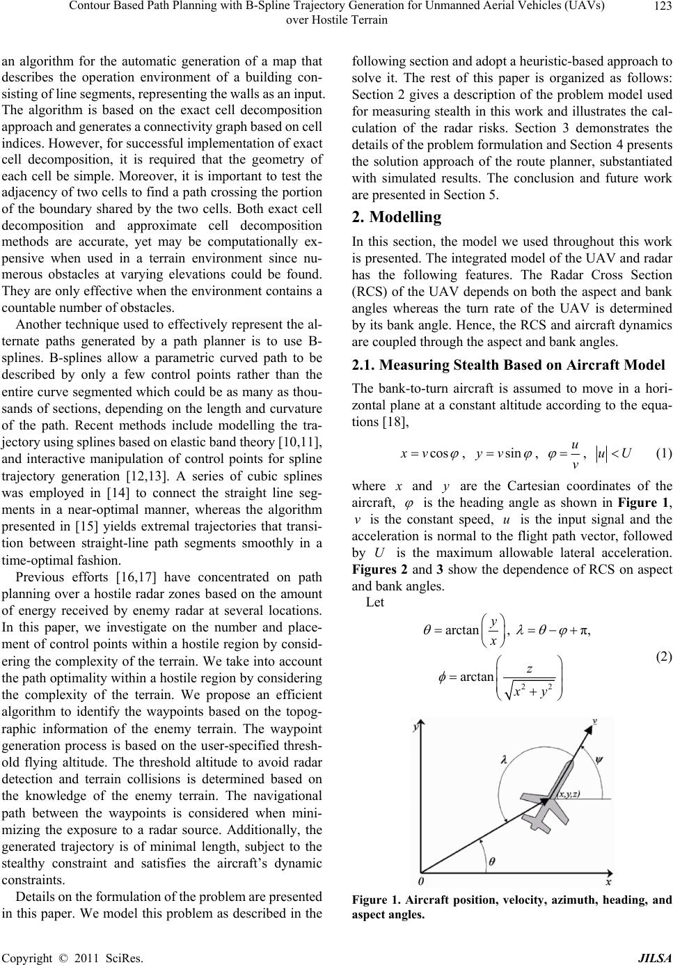

Contour Based Path Planning with B-Spline Trajectory Generation for Unmanned Aerial Vehicles (UAVs) 123
over Hostile Terrain
an algorithm for the automatic generation of a map that
describes the operation environment of a building con-
sisting of line segments, representing the walls as an input.
The algorithm is based on the exact cell decomposition
approach and generates a connectivity graph based on cell
indices. However, for successful implementation of exact
cell decomposition, it is required that the geometry of
each cell be simple. Moreover, it is important to test the
adjacency of two cells to find a path crossing the portion
of the boundary shared by the two cells. Both exact cell
decomposition and approximate cell decomposition
methods are accurate, yet may be computationally ex-
pensive when used in a terrain environment since nu-
merous obstacles at varying elevations could be found.
They are only effective when the environment contains a
countable number of obstacles.
Another technique used to effectively represent the al-
ternate paths generated by a path planner is to use B-
splines. B-splines allow a parametric curved path to be
described by only a few control points rather than the
entire curve segmented which could be as many as thou-
sands of sections, depending on the length and curvature
of the path. Recent methods include modelling the tra-
jectory using splines based on elastic band theory [10,11],
and interactive manipulation of control points for spline
trajectory generation [12,13]. A series of cubic splines
was employed in [14] to connect the straight line seg-
ments in a near-optimal manner, whereas the algorithm
presented in [15] yields extremal trajectories that transi-
tion between straight-line path segments smoothly in a
time-optimal fashion.
Previous efforts [16,17] have concentrated on path
planning over a hostile radar zonesbased on the amount
of energy received by enemy radar at several locations.
In this paper, we investigate on the number and place-
ment of control points within a hostile region by consid-
ering the complexity of the terrain. We take into account
the path optimality within a hostile region by considering
the complexity of the terrain. We propose an efficient
algorithm to identify the waypoints based on the topog-
raphic information of the enemy terrain. The waypoint
generation process is based on the user-specified thresh-
old flying altitude. The threshold altitude to avoid radar
detection and terrain collisions is determined based on
the knowledge of the enemy terrain. The navigational
path between the waypoints is considered when mini-
mizing the exposure to a radar source. Additionally, the
generated trajectory is of minimal length, subject to the
stealthy constraint and satisfies the aircraft’s dynamic
constraints.
Details on the formulation of the problem are presented
in this paper. We model this problem as described in the
following section and adopt a heuristic-based approach to
solve it. The rest of this paper is organized as follows:
Section 2 gives a description of the problem model used
for measuring stealth in this work and illustrates the cal-
culation of the radar risks. Section 3 demonstrates the
details of the problem formulation and Section 4 presents
the solution approach of the route planner, substantiated
with simulated results. The conclusion and future work
are presented in Section 5.
2. Modelling
In this section, the model we used throughout this work
is presented. The integrated model of the UAV and radar
has the following features. The Radar Cross Section
(RCS) of the UAV depends on both the aspect and bank
angles whereas the turn rate of the UAV is determined
by its bank angle. Hence, the RCS and aircraft dynamics
are coupled through the aspect and bank angles.
2.1. Measuring Stealth Based on Aircraft Model
The bank-to-turn aircraft is assumed to move in a hori-
zontal plane at a constant altitude according to the equa-
tions [18],
cos
x
v


, sinyv


, u
v
 , uU

(1)
where
x
and are the Cartesian coordinates of the
aircraft,
y

is the heading angle as shown in Figure 1,
is the constant speed, is the input signal and the
acceleration is normal to the flight path vector, followed
by is the maximum allowable lateral acceleration.
Figures 2 and 3 show the dependence of RCS on aspect
and bank angles.
vu
U
Let
22
arctan, π,
arctan
y
x
z
xy











 
(2)
Figure 1. Aircraft position, velocity, azimuth, heading, and
aspect angles.

Contour Based Path Planning with B-Spline Trajectory Generation for Unmanned Aerial Vehicles (UAVs) 124
over Hostile Terrain
Figure 2. RCS as a function of aspect angle.
Figure 3. RCS as a function of bank angle.
be the azimuth, aspect, and elevation angles, respectively,
where z is the aircraft altitude. Let the bank angle μ be
given by
arctan u u
g



(3)
where g is the acceleration of gravity. We model the
RCS of the aircraft as function of the aspect angle λ, the
elevation angle φ, and the bank angle μ, so that
RCS =

RCS, ,


  (4)
The RCS obtained from Equation (4) is used as an es-
timate value in Equation (6) for measuring stealth in this
work. As an example, real aircraft RCS measurements as
functions of aspect and bank angles are shown in Fig-
ures 3 and 4 [18]. The following section illustrates the
calculation of the cost associated to radar risk that will be
undertaken by the UAV.
2.2. Radar Model
The radar model in this work will be presented in terms
of its inputs (aircraft range and RCS) and output (an es-
timate of the probability that an aircraft can be tracked
for an interval of time). For the sake of simplicity, we
assume that the radar is located at (
x
,, ) of the navi-
gational space. Let
y z
Figure 4. Square cylinder for RCS modelling.

22
Rxyz 2 (5)
be the aircraft range from the enemy radar to the aircraft.
The radar detects the aircraft by receiving a sequence of
radio frequency pulses reflected from it at fixed observa-
tion times. To generate a stealthy path for the UAV, we
have to take into account the energy reflected to enemy
radar site as the enemy radar tracks the location, speed,
and direction of an aircraft. The range at which radar can
detect an object is related to the power transmitted by the
radar, the fidelity of the radar antenna, the wavelength of
the radar signal, and the RCS of the aircraft [19]. The
RCS is the area a target would have to occupy to produce
the amount of reflected power that is detected back at the
radar. RCS is integral to the development of radar stealth
technology, particularly in applications involving aircraft.
For example, a stealth aircraft which is designed to be
undetectable will have design features that give it a low
RCS. Low RCS offers advantages in detection range
reduction as well as increasing the effectiveness of de-
coys against radar-seeking threats. The size of a target's
image on radar is measured by the RCS and denoted by
the symbol σ and expressed in square meters. The azi-
muth and range detected by the radar serve as the inputs
to a tracking system, typically based on one or more
Kalman filters. The purpose of the tracking system is to
provide a predicted aircraft position and velocity so that
a decision can be made to launch a missile and guide it to
intercept. RCS modelling and reduction is crucial in de-
signing stealth weapon systems. We make use of Finite-
Difference Time-Domain (FDTD) Method technique in
RCS modelling. The numerical technique is general,
geometry-free, and can be used arbitrarily for any target,
within the limitations of computer memory and speed.
Figure 4 shows the geometric surface for the RCS simu-
lation with the FDTD algorithm. The FDTD-based
package was supplied in [20] for the RCS prediction of
C opyright © 2011 SciRes. JILSA

Contour Based Path Planning with B-Spline Trajectory Generation for Unmanned Aerial Vehicles (UAVs) 125
over Hostile Terrain
various simple canonical targets. The complete RCS
signature of a target is described by the frequency re-
sponse of the target illuminated by plane waves from all
possible physical angles. Realistic targets are frequently
very large and are often largely made up of highly con-
ductive materials.
The FDTD-based RCS prediction procedure is as fol-
lows:
 The target, located in the computational space, is illu-
minated by a Gaussian-pulse plane wave from a given
direction;
 The scattered fields are simulated inside the computa-
tional volume until all transients dissipate;
 The time-domain far fields in the spherical coordinates
are then extrapolated by using equivalent current via
the near-field to far-field routine, over a closed, virtual
surface surrounding the target.
For either vertical or horizontal planes, co-polarized or
cross-polarized RCS behaviour is computed after the
simulation for a given frequency range. Figure 5 illus-
trates the RCS behaviour with respect to the azimuth
angle based on the RCS modelling described above.
Subsequently the computation of the energy received
by a radar is given by the radar range equation [21]

24
4π
avgot e
PGtA
SR

 (6)
where S is the signal energy received by the radar, Pavg is
the average power transmitted by the radar, G is the gain
of the radar antenna, σ is the radar cross section of the
target, Ae is the effective area of the radar antenna, tot is
the time the radar antenna is pointed at the target, and R
is the range to the target. Every radar has a minimum
signal energy that it can detect, Smin. This minimum sig-
nal energy determines the maximum range (Rmax) at
which the radar can detect a given target.

4
max 2
min
4π
avge ot
PGAt
RS

 (7)
Figure 5. RCS behaviour with respect to the azimuth angle.
According to Equation (7), the distance at which a tar-
get can be detected for given radar configuration varies
with the fourth root of its RCS. Figure 6 gives some
understanding of just how little radar power is typically
reflected back from the target and received by the radar.
In this case, the target presents the same aspect to the
radar at ranges from 1 to 50 miles. At a range of 50 miles,
the relative power received by the radar is only 1.6 ×
10–5% of the strength at one mile. This diagram graphi-
cally illustrates how significant the effect of energy dis-
sipation is with distance, and how sensitive radars must
be to detect targets at even short ranges. Hence the cost
associated to radar risk is based on a UAV’s exposure to
enemy radar. In this work, the cost of radar risk involves
the amount of energy received by enemy radar at several
locations based on the distance between the UAV and the
radar. We assume that the UAV’s radar signature is uni-
form in all directions and is proportional to 1/R4 (where
R is the distance between the UAV and the enemy radar);
the UAVs are assigned simplified flight dynamics and
performance constraints in two-dimensions; and all
tracking radars are given simplified detection properties.
Based on the assumptions stated above, we classify the
navigational space into different levels of risk as de-
scribed in the following chapter. The next step is to
compute a stealthy path, steering the UAV clear and
around known radar locations. The generated path should
carry minimal radar risks, and adhere to physical and
motion constraints. Also, the distance between the UAV
and the radars should be maximized in order to minimize
the energy received at the radar.
3. Problem Formulation
To describe the problem, consider the contour based
navigational space shown in Figure 7. The objective is
to find a path which minimizes the UAV’s exposure to
radar sites (small triangles) from the current UAV posi-
tion (circle) to the target location (star). In the present
study, it is assumed that the hostile radar zones are
Figure 6. Reduction in the strength of target echoes with
range.

Contour Based Path Planning with B-Spline Trajectory Generation for Unmanned Aerial Vehicles (UAVs) 126
over Hostile Terrain
Figure 7. Contour based navigational space with known
radar sites.
known beforehand. The contours are used to denote ele-
vation and depth on maps. From these contours, a sense
of the general terrain can be determined. The details of
the radar zone can be acquired using satellite data or
from surveillance data. The start point and the end point
of the flight are known and it is required to find a feasi-
ble path connecting these two points. The threshold alti-
tude value is determined by the user which assumes
knowledge of the enemy terrain. By flying at a user-
specified threshold altitude value, the aircraft can take
advantage of terrain masking and avoid detection by
enemy radars. The aircraft works by transmitting a radar
signal towards the ground area and the signal returns can
then be analysed to see how the terrain ahead varies,
which can then be used by the aircraft's autopilot to
specify the threshold altitude value. The specified thresh-
old allows the aircraft to fly at reasonably constant height
above the earth so as to avoid the radar detection. In this
work, the path of the UAV is smoothened using cubic B-
splines, which is controlled by manipulating a number of
control points. The generated path should carry minimal
radar risks, and adhere to physical and motion con-
straints.
Given a single radar located at the origin and a single
aircraft travelling from initial point to the destination,
Pachter [22] showed that an objective function for mini-
mizing cost, is

4
0
1d
l
v
J
t
Rt
 (8)
where v is the constant speed of the aircraft and l is the
path length. A closed form solution to this problem was
obtained using the calculus of variations, with the limita-
tion that the aircraft traverses an angle with respect to the
radar of less than 60˚. Beyond this limit, the optimal path
length is infinite but the cost remains finite. The objec-
tive cost function Equation (8), is augmented to include
the rest of the radar at the navigational space, giving

4 1
0d
lmi
v
i
J
t
Rt



 (9)
The cost associated with radar risk involves the amount
of energy i

, received by enemy radar based on the
distance from the UAV to the radar. We first look for
appropriate waypoints that the UAV should traverse in
planning a path which minimizes the radar exposure.
4. Generation of Nodes
The procedure starts by requesting from the user the de-
tection altitude or maximum elevation desired which
assumes knowledge of the enemy terrain. Nodes below
the detection altitude are extracted and used as base in
the generation of straight line segments. The nodes above
the detection altitude are discarded, given that at those
elevations the UAVs could be detected. Appropriate
value for the parameter is based on the user’s knowledge
of: the terrain; the operation of the UAVs; the purpose,
logistics, and safety of the mission. This means that the
user’s input is a determinant in the quality of the result-
ing path. As shown in Figure 8, the initial nodes can be
searched by specifying the detection altitude for the
UAV. The next step is to make use of heuristic search
algorithm to compute a stealthy path, steering the UAV
clear and around known radar locations.
5. Implementation
5.1. Generation of Nodes
This search algorithm works by starting at UAV’s pre-
Figure 8. Generated waypoints based on user-specified
threshold altitude value.
C opyright © 2011 SciRes. JILSA

Contour Based Path Planning with B-Spline Trajectory Generation for Unmanned Aerial Vehicles (UAVs) 127
over Hostile Terrain
sent position (red circle). It adds the heuristic function
value and determines the expansion order of nodes. We
make use of a distance-plus-cost heuristic function, f(n)
to determine the order in which the search visits nodes in
the space. We assume that the UAV’s radar signature is
uniform in all directions and is proportional to 1/R4
where R is the aircraft range. We modify the evaluation
function by adding the cost associated with radar risk to
the f(n) as follows:
 
4 0
1mi
i
i
c
fnwgnw hnR

 
 (10)
where w is a value in the range [0, 1]; g(n) is the path-
cost function which shows the intensity between the cur-
rent node and node n; h(n) is the distance value which is
estimated from node n to the goal node; ci is relative to Ri
and m is the number of enemy radars located at the
navigational space. The h(n) plays a significant role in
the search process when w value is smaller; the number
of vertices to be explored would be decreased. The
choice of w between 0 and 1 gives the flexibility to place
weight on exposure to threats or fuel expenditure de-
pending on the particular mission scenario. For example
when w = 0, the search process would proceed from the
starting location to the target location by exploring the
least number of vertices. However the generated path is
not stealthy and may cause UAV to enter high radar risk
region. A w value closer to 0 would result in the shortest
paths, with little regard for the exposure to enemy radar,
while a value closer to 1 would result in paths that avoid
threat exposure at the expense of longer path length. For
this case, the cost weighting parameter w was chosen to
give a reasonable tradeoff between proximity of the path
to threats and the path length. The evaluation function,
(10) is tested empirically and compared in terms of the
number of nodes visited. During the test, the cost
weighting parameter w is varied from 0.0 to 1.0 and the
test result is demonstrated in Table 1. The experimen-
tally defined value for the w ranges from [0.1, 0.3] in
which the generated path is optimal and computationally
inexpensive, which is in line with our algorithm objec-
tives. The generated path is neither the safest possible
path nor the shortest possible path, but represents a com-
promise between the two objectives.
The algorithm traverses various paths from the starting
location to the goal. At the same time, it compares the
risk cost of all the vertices. Starting with the initial node,
it maintains a priority queue of nodes to be traversed,
known as the openQueue (see Listing 1). The lower f(n)
for a given node n, the higher its priority. At each step of
the algorithm, the node with the lowest f(n) value is re-
moved from the queue, the f and h values of its neighbors
Table 1. Test results.
Cost Weighting Pa-
rameter, w Explored Nodes Cost of the Generated Path
w is not used 2405 103
0 385 117.5
0.1 369 112.5
0.2 365 110.5
0.3 365 106.5
0.4 468 104
0.5 2405 103
0.6 4975 101
0.7 7073 100.5
0.8 7521 99
0.9 7766 97
1.0 8085 97
The algorithm traverses various paths from the starting
location to the goal. At the same time, it compares the
risk cost of all the vertices. Starting with the initial node,
it maintains a priority queue of nodes to be traversed,
known as the openQueue (see Listing 1). The lower f(n)
for a given node n, the higher its priority. At each step of
the algorithm, the node with the lowest f(n) value is re-
moved from the queue, the f and h values of its neighbors
are updated accordingly, and these neighbors with the
least radar cost are added to the openQueue. The condi-
tions of adding a node to the openQueue are as follows:
 The node is not in high radar risk region;
 The node is movable and does not exist in the open-
Queue;
 The distance between the starting point and the current
node is shorter than the earlier estimated distance;
 The distance between the starting point and the current
node does not violate the pre-specified detection alti-
tude.
If the four conditions are satisfied, then the current
node will be added to the openQueue. The algorithm
continues until a goal node has a lower f value than any
node in the queue. If the actual optimal path is desired,
the algorithm may also update each neighbor with its
immediate predecessor in the best path found so far; this
information can then be used to reconstruct the path by
working backwards from the goal node. The output of
this stage is a set of straight line segments connecting a
subset of the nodes resulting from the waypoint genera-
tion process, as long as the link does not violate the
pre-specified detection altitude. The path planning algo-
rithm is implemented in a MATLAB environment and a
sample of the result can be seen in Figure 9.
The pseudo-code for the algorithm is as shown in
Listing 1.
The next step is to modify the generated path by using
a series of cubic splines to optimize the path by moving
away from high radar risks and improving the navigabil-
ity of the path for the UAV.

Contour Based Path Planning with B-Spline Trajectory Generation for Unmanned Aerial Vehicles (UAVs) 128
over Hostile Terrain
Figure 9. Generated path with least radar risk based on
user-specified detection altitude.
5.2. Trajectory Generation
As a first step, the path is parameterized in both x and
y directions. An initial spline knot is fixed at the UAV
starting location, while the final spline knot is fixed at
the first edge of the path. We begin by splitting each
edge of the path into three segments, each one described
by a different B-spline curve [23]. In this work, we
calculate the radar risk cost at several locations along
each edge and take the length of the edge into account.
The radar risk cost was calculated at three points along
each edge: Li/6, Li/2, and 5Li/6, where Li is the length of
edge i. The radar risk cost for each edge may be calcu-
lated by
444 11
16,, 12,, 56,,
111 NM
ei
ji
ij ijij
JL ddd j



 


 (11)
where N is the number of enemy radars; M is the number
of discrete point and d1/6,i,j is the distance from the 1/6th
point on the ith edge to the jth enemy radar. The goal now
is to find the (x, y) locations which minimize the
exposure to the enemy radar for the middle knots. We
apply the graph search algorithm to look for the middle
knots with minimal risk cost for each edge of the path.
We determine the interpolating curve based on tangent
vectors and curvature vectors for each pair of points. The
interpolation problem is solved by assuming p = 3, which
produces the C2 cubic spline [24]. The parameters ûk are
used to determine the knot vector u as
0120
ˆ,uuuu
3ˆ jj
uu

456
ˆ,
nnn
uuuu


,0, ,jn
n

 (12)
Since the number of control points, m + 1, and the
number of the knots, nknot + 1, are related by nknot = m + 4
and, as can be easily deduced from (12), nknot = n + 6, the
Function search_path (start, goal)
closedQueue: = the empty queue/*The set of nodes
already evaluated*/
openQueue: = queue containing the initial node/
*The set of tentative nodes to be evaluated*/
g[start]: = 0/*Distance from start along optimal
path*/
h[start]: = estimate_of_distance (start, goal)
f[start]:= h[start]/*Estimated total distance from
start to goal through y*/
while openQueue is not empty
n: = the node in openQueue having the lowest
f[] value
if n = goal
return reconstruct_path (came_from, goal)
remove n from openQueue
add n to closedQueue
for each y in neighbor_nodes (n)
if y in closedQueue
continue
tentative_g: = g [n] + dist_between (n, y) +
risk_cost
/*Compares the risk cost*/
tentative_is_better:= false
if y not in openQueue
add y to openQueue
h[y]: = estimate_of_distance (y, goal)
tentative_is_better:= true
elseif tentative_g < g[y]
tentative_is_better: = true
if tentative_is_better = true
came_from[y]: = n
g[y]: = tentative_g
f[y]: = g[y] + h[y]
return failure
function reconstruct_path (came_from,current_node)
if came_from[current_node ] is set p = recon-
struct_path (came_from, came_from[current_node])
return (p + current_node)
else
return the empty path
Listing 1. Pseudo-code for the path planning algorithm.
unknown variables pj are n + 3. Once the control points
pj, j = 0, , n + 2 are known, and given the knot vector
u, the B-spline is completely defined. Once this step has
been completed, the procedure switches to the algorithm
(as shown in List ing 2) to determine how to connect the
knots. Note that some experimentally defined knots are
added by the algorithm in order to smoothen the spline
curve.

C opyright © 2011 SciRes. JILSA

Contour Based Path Planning with B-Spline Trajectory Generation for Unmanned Aerial Vehicles (UAVs) 129
over Hostile Terrain
Listing 2. Pseudo-code for generating a spline path.
It is worth noticing that the interpolation by means of
cubic B-splines guarantees the C2 continuity of the
geometric path. Owing to the continuity of the curve
derivatives, it is not possible to obtain a path with sharp
corners that is not flyable by the UAVs. An illustration
of the generated solution is shown in Figure 10.
6. Conclusions and Future Works
This paper presents a contour based path planner to gen-
erate an optimal path for UAVs over hostile terrain. The
proposed method is flexible given that it allows the user
to input a threshold altitude value to avoid radar detec-
tion and terrain collisions. The key strengths of the
method are: 1) the ability to plot a safe path to the target
while minimizing exposure to the enemy radar; 2) the
generated paths are smoothened using cubic splines to
Figure 10. Optimal path based on heuristic search algo-
rithm and user-specified threshold altitude.
improve navigability and 3) computational efficiency is
achieved. Using this planning approach, the ability to
generate feasible paths has been demonstrated through
simulations. The information provided in this paper is
significant for the planning of an air reconnaissance mis-
sion. However the procedure has limitations and is sensi-
tive to some of the input parameters, leaving room for
improvements in future research based on computational
intelligence approaches [25-28].
7. Acknowledgements
The authors gratefully acknowledge the funding support
from Temasek Defence Systems Institute, Singapore.
8. References
Function spline_path (start, goal)
locate_points()/*get coordinates (x, y) of middle
knots*/
m_points: = the vector list/* to store control
points*/
m_nodes: = the vector list/* to store small nodes*/
m_steps: = number of steps/*steps for spline*/
add_points (x, y)/*store (x, y) in a vector list*/
while (x, y) is not goal
new_controlpoint_added ()
/*spline curve based on the control points and
nodes*/
for int i = 0 to m_steps
compute blending function

1
32
1
2
13 31
3630
1
130 30
6
1410
i
i
i
i
i
p
p
t
tttp
p








 


 



 


 



S
for


0, 1t
get_point (double u, const GLVector & P0,
const GLVector & P1, const GLVector & P2, const
GLVector & P3)
/*return coordinate (x, y) for particular t*/
add_node (const GLVector & node)/*add
small nodes in between the control points and we
make use of 100 small nodes in this work*/
end for
end while
render_spline()/*display generated curve*/
return the spline path
[1] A. Agarwal, M. H. Lim, M. J. Er and T. N. Nguyen,
“Rectilinear Workspace Partitioning for Parallel Cover-
age Using Multiple UAVs,” Advanced Robotics, Vol.
21, No. 1, 2007, pp. 105-120.
[2] K. K. Lim, Y. S. Ong, M. H. Lim and A. Agarwal, “Hy-
brid Ant Colony Algorithm for Path Planning in Sparse
Graphs,” Soft Computing Journal, Vol. 12, No. 10, 2008,
pp. 981-994.
[3] C. W. Yeu, M. H. Lim, G. Huang, A. Agarwal and Y. S.
Ong, “A New Machine Learning Paradigm for Terrain
Reconstruction,” IEEE Geoscience and Remote Sensing
Letters, Vol. 3, No. 3, 2006, pp. 981-994.
doi:10.1109/LGRS.2006.873687
[4] L. Davis, “Warp Speed: Path Planning for Star Trek:
Armada,” AAAI Spring Symposium, AAAI Press, Menlo
Park, 2000.
[5] E. Frazzoli, M. Dahleh and E. Feron, “Real-Time Motion
Planning for Agile Autonomous Vehicles,” Journal of
Guidance, Control and Dynamics, Vol. 25, No. 1, 2002,
pp. 116-129. doi:10.2514/2.4856

Contour Based Path Planning with B-Spline Trajectory Generation for Unmanned Aerial Vehicles (UAVs)
over Hostile Terrain
130
[6] N. H. Sleumer and N. Tschichold-Gürman, “Exact Cell
Decomposition of Arrangements Used for Path Planning
in Robotics,” Technical Reports 329, ETH Zürich, Insti-
tute of Theoretical Computer Science, 1999.
[7] J. C. Latombe, “Robot Motion Planning,” Kulwer Aca-
demic Publishers, Boston, 1991.
[8] T. Lozano-Pyrez and M. A. Wesley, “An Algorithm for
Planning Collision-Free Paths among Polyhedral Obsta-
cles,” Communications of the ACM, Vo1. 22, No. 10,
1979, pp. 565-570.
[9] M. Jun, “Path Planning for Unmanned Aerial Vehicles in
Uncertain and Adversarial Environments,” In: S. Butenko,
R. Murphey and P. Pardalos, Eds., Cooperative Control:
Models, Applicarions and Algorithms, Kluwer, 2003, pp.
95-111.
[10] J. Hilgert, K. Hirsch, T. Bertram and M. Hiller, “Emer-
gency Path Planning for AutonomousVehicles Using
Elastic Band Theory,” Advanced Intelligent Mechatronics,
Vol. 2, 2003, pp. 1390-1395.
[11] T. Sattel and T. Brandt, “Ground Vehicle Guidance
Along Collision-Free Trajectories Using Elastic Bands,”
Proceedings of 2005 American Control Conference, Port-
la, 2005, pp. 4991-4999.
[12] J. Hwang, R. C. Arkin and D. Kwon, “Mobile Robots at
Your Fingertip: Bezier Curve On-Line Trajectory Gen-
eration for Supervisory Control,” Proceedings of Intelli-
gent Robots and Systems (IROS 2003), Las Vegas, Vol. 2,
2003, pp. 1444-1449.
[13] J. Aleotti, S. Caselli and G. Maccherozzi, “Trajectory
Reconstruction with NURBS Curves for Robot Pro-
gramming by Demonstration,” Proceedings of Computa-
tional Intelligence in Robotics and Automation, Barce-
lona, 2005, pp. 73-78.
[14] K. B. Judd and T. W. McLain, “Spline Based Path Plan-
ning for Unmanned Air Vehicles,” AIAA Guidance,
Navigation, and Control Conference and Exhibit, Mont-
real, 2001.
[15] E. P. Anderson, R. W. Beard, and T. W. McLain, “Real-
Time Dynamic Trajectory Smoothing for Unmanned Air
Vehicles,” IEEE Transactions on Control Systems Tech-
nology, Vol. 13, No. 3, 2005, pp. 471-477.
doi:10.1109/TCST.2004.839555
[16] E. M. Kan, M. H. Lim, S. P. Yeo, S. H. Shao and J. S. Ho,
“Radar Aware Path Planning for UAVs,” IEEE Sympo-
sium on Intelligent Systems and Applications, Trabzon,
June 2009.
[17] E. M. Kan, S. P. Yeo, C. S.Tan, S. H. Shao and J. S. Ho,
“Stealth Path Planning for UAVs in Hostile Radar
Zones,” Proceedings of the 11th IASTED International
Conference on Control and Applications, Cambridge,
July 2009, pp. 54-60.
[18] F. W. Moore, “Radar Cross-Section Reduction via Route
Planning and Intelligent Control,” IEEE Transactions on
Control Systems Technology, Vol. 10, No. 5, 2002, pp.
696-700. doi:10.1109/TCST.2002.801879
[19] U. F. Knott, “Radar Cross Section Measurements,” Van
Nostrand Reinhold, New York, 1993.
[20] L. Sevgi, “Complex Electromagnetic Problems and Nu-
merical Simulation Approaches,” IEEE Press/John Wiley
& Sons, New York, 2003.
[21] E. F. Knott, J. F. Shaeffer, and M. T. Tuley, “Radar Cross
Section,” 2nd Edition, Artech House, Norwood, 1993, p.
231.
[22] M. Pachter, D. R. Jacques and J. M. Hebert, “Minimizing
Radar Exposure in Air Vehicle Path Planning,” Proceed-
ings of the 41st Israel Annual Conference on Aerospace
Sciences, Tel-Aviv, February 2001.
[23] M. G. Cox, “The Numerical Evaluation of B-Splines,”
IMA Journal of Applied Mathematics, Vol. 10, No. 2,
1972, pp. 134-149. doi:10.1093/imamat/10.2.134
[24] R. H. Bartels, J. C. Beatty and B. A. Barsky, “An Intro-
duction to Splines for Use in Computer Graphics and
Geometric Modeling,” Morgan Kaufmann Publishers,
Massachusetts, 1987.
[25] Q. Cao, M. H. Lim, J. H. Li, Y. S. Ong and W. L. Ng, “A
Context Switchable Fuzzy Inference Chip,” IEEE Trans-
actions on Fuzzy Systems, Vol. 14, No. 4, 2006, pp. 552-
567. doi:10.1109/TFUZZ.2006.876735
[26] M. H. Lim and Y Takefuji, “Implementing Fuzzy Rule-
Based Systems on Silicon Chips,” IEEE Expert, Vol. 5,
No. 1, 1990, pp. 31-45. doi:10.1109/64.50855
[27] R. Meuth, M. H. Lim, Y. S. Ong and D. C. Wunsh, “A
Proposition on Memes and Meta-Memes in Computing
for Higher-Order Learning,” Memetic Computing, Vol. 1,
No. 2, 2009, pp. 85-100. doi:10.1007/s12293-009-0011-1
[28] M. H. Lim, Q. Cao, J. H. Li and W. L. Ng, “Evolvable
Hardware Using Context Switchable Fuzzy Inference
Processor,” IEEE Proceedings: Computers and Digital
Techniques, Vol. 151, No. 4, 2004, pp. 301-311.
doi:10.1049/ip-cdt:20040666
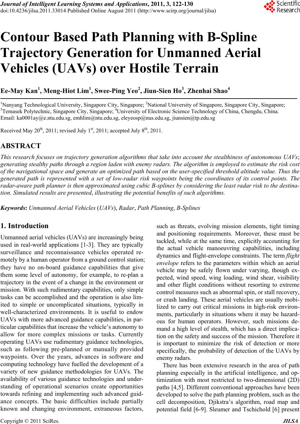