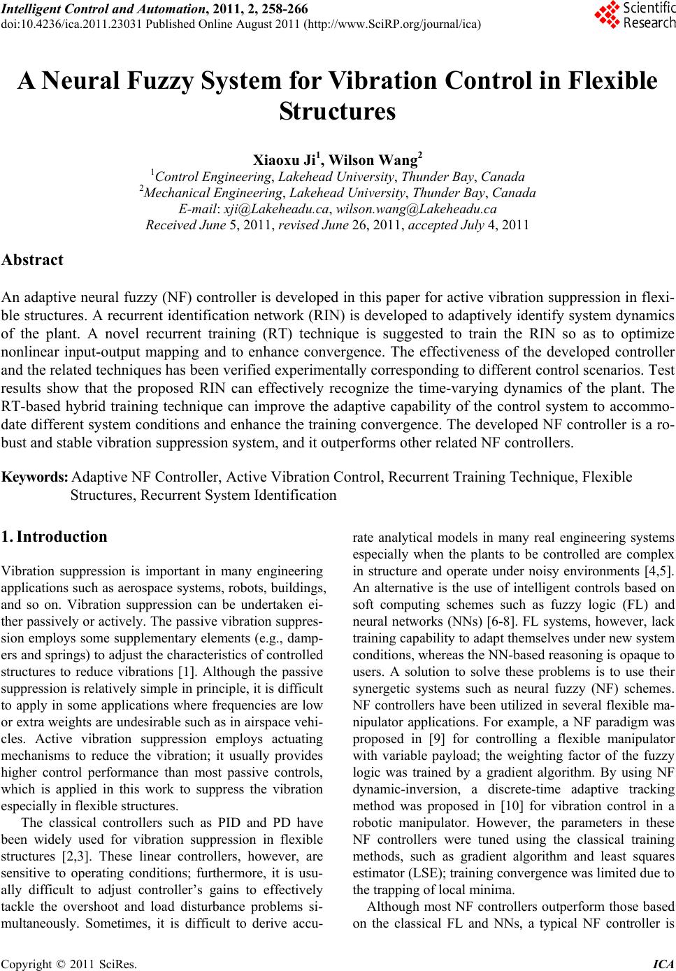
Intelligent Control and Automation, 2011, 2, 258-266
doi:10.4236/ica.2011.23031 Published Online August 2011 (http://www.SciRP.org/journal/ica)
A Neural Fuzzy System for Vibration Control in Flexible
Structures
Xiaoxu Ji1, Wilson Wang2
1Control Engineering, Lakehead University, Thunder Bay, Canada
2Mechanical Engineering, Lakehead University, Thunder Bay, Canada
Received June 5, 2011, revised June 26, 2011, accepted July 4, 2011
Abstract
An adaptive neural fuzzy (NF) controller is developed in this paper for active vibration suppression in flexi-
ble structures. A recurrent identification network (RIN) is developed to adaptively identify system dynamics
of the plant. A novel recurrent training (RT) technique is suggested to train the RIN so as to optimize
nonlinear input-output mapping and to enhance convergence. The effectiveness of the developed controller
and the related techniques has been verified experimentally corresponding to different control scenarios. Test
results show that the proposed RIN can effectively recognize the time-varying dynamics of the plant. The
RT-based hybrid training technique can improve the adaptive capability of the control system to accommo-
date different system conditions and enhance the training convergence. The developed NF controller is a ro-
bust and stable vibration suppression system, and it outperforms other related NF controllers.
Keywords: Adaptive NF Controller, Active Vibration Control, Recurrent Training Technique, Flexible
Structures, Recurrent System Identification
1. Introduction
Vibration suppression is important in many engineering
applications such as aerospace systems, robots, buildings,
and so on. Vibration suppression can be undertaken ei-
ther passively or actively. The passive vibration suppres-
sion employs some supplementary elements (e.g., damp-
ers and springs) to adjust the characteristics of controlled
structures to reduce vibrations [1]. Although the passive
suppression is relatively simple in principle, it is difficult
to apply in some applications where frequencies are low
or extra weights are undesirable such as in airspace vehi-
cles. Active vibration suppression employs actuating
mechanisms to reduce the vibration; it usually provides
higher control performance than most passive controls,
which is applied in this work to suppress the vibration
especially in flexible structures.
The classical controllers such as PID and PD have
been widely used for vibration suppression in flexible
structures [2,3]. These linear controllers, however, are
sensitive to operating conditions; furthermore, it is usu-
ally difficult to adjust controller’s gains to effectively
tackle the overshoot and load disturbance problems si-
multaneously. Sometimes, it is difficult to derive accu-
rate analytical models in many real engineering systems
especially when the plants to be controlled are complex
in structure and operate under noisy environments [4,5].
An alternative is the use of intelligent controls based on
soft computing schemes such as fuzzy logic (FL) and
neural networks (NNs) [6-8]. FL systems, however, lack
training capability to adapt themselves under new system
conditions, whereas the NN-based reasoning is opaque to
users. A solution to solve these problems is to use their
synergetic systems such as neural fuzzy (NF) schemes.
NF controllers have been utilized in several flexible ma-
nipulator applications. For example, a NF paradigm was
proposed in [9] for controlling a flexible manipulator
with variable payload; the weighting factor of the fuzzy
logic was trained by a gradient algorithm. By using NF
dynamic-inversion, a discrete-time adaptive tracking
method was proposed in [10] for vibration control in a
robotic manipulator. However, the parameters in these
NF controllers were tuned using the classical training
methods, such as gradient algorithm and least squares
estimator (LSE); training convergence was limited due to
the trapping of local minima.
Although most NF controllers outperform those based
on the classical FL and NNs, a typical NF controller is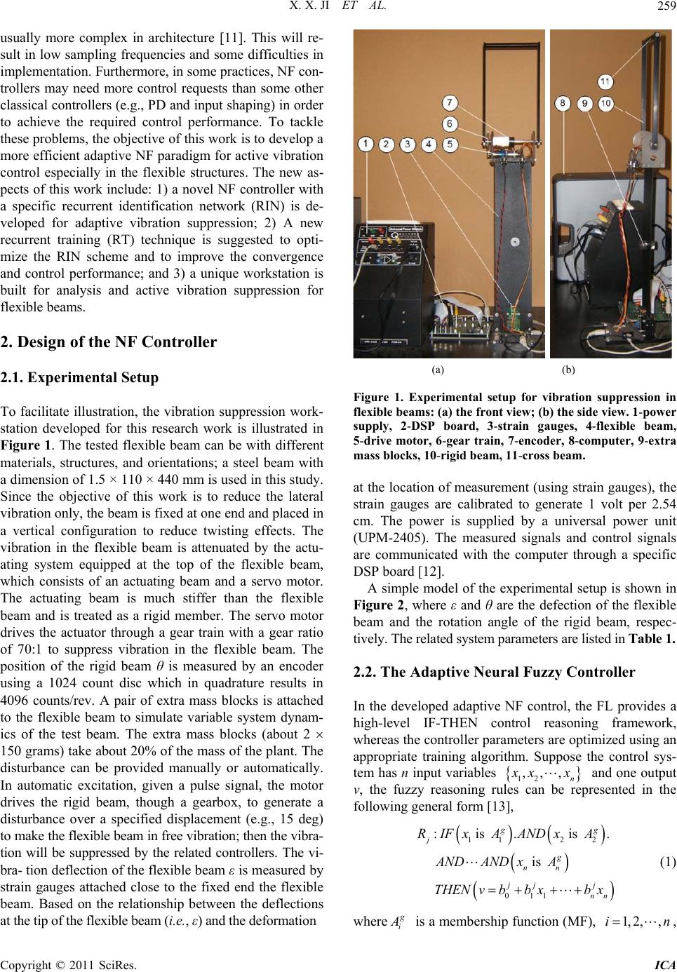

X. X. JI ET AL.259
usually more complex in architecture [11]. This will re-
sult in low sampling frequencies and some difficulties in
implementation. Furthermore, in some practices, NF con-
trollers may need more control requests than some other
classical controllers (e.g., PD and input shaping) in order
to achieve the required control performance. To tackle
these problems, the objective of this work is to develop a
more efficient adaptive NF paradigm for active vibration
control especially in the flexible structures. The new as-
pects of this work include: 1) a novel NF controller with
a specific recurrent identification network (RIN) is de-
veloped for adaptive vibration suppression; 2) A new
recurrent training (RT) technique is suggested to opti-
mize the RIN scheme and to improve the convergence
and control performance; and 3) a unique workstation is
built for analysis and active vibration suppression for
flexible beams.
2. Design of the NF Controller
2.1. Experimental Setup
To facilitate illustration, the vibration suppression work-
station developed for this research work is illustrated in
Figure 1. The tested flexible beam can be with different
materials, structures, and orientations; a steel beam with
a dimension of 1.5 × 110 × 440 mm is used in this study.
Since the objective of this work is to reduce the lateral
vibration only, the beam is fixed at one end and placed in
a vertical configuration to reduce twisting effects. The
vibration in the flexible beam is attenuated by the actu-
ating system equipped at the top of the flexible beam,
which consists of an actuating beam and a servo motor.
The actuating beam is much stiffer than the flexible
beam and is treated as a rigid member. The servo motor
drives the actuator through a gear train with a gear ratio
of 70:1 to suppress vibration in the flexible beam. The
position of the rigid beam θ is measured by an encoder
using a 1024 count disc which in quadrature results in
4096 counts/rev. A pair of extra mass blocks is attached
to the flexible beam to simulate variable system dynam-
ics of the test beam. The extra mass blocks (about 2 
150 grams) take about 20% of the mass of the plant. The
disturbance can be provided manually or automatically.
In automatic excitation, given a pulse signal, the motor
drives the rigid beam, though a gearbox, to generate a
disturbance over a specified displacement (e.g., 15 deg)
to make the flexible beam in free vibration; then the vibra-
tion will be suppressed by the related controllers. The vi-
bra- tion deflection of the flexible beam ε is measured by
strain gauges attached close to the fixed end the flexible
beam. Based on the relationship between the deflections
at the tip of the flexible beam (i.e., ε) and the deformation
(a) (b)
Figure 1. Experimental setup for vibration suppression in
flexible beams: (a) the front view; (b) the side view. 1-power
supply, 2-DSP board, 3-strain gauges, 4-flexible beam,
5-drive motor, 6-gear train, 7-encoder, 8-computer, 9-extra
mass blocks, 10-rigid beam, 11-cross beam.
at the location of measurement (using strain gauges), the
strain gauges are calibrated to generate 1 volt per 2.54
cm. The power is supplied by a universal power unit
(UPM-2405). The measured signals and control signals
are communicated with the computer through a specific
DSP board [12].
A simple model of the experimental setup is shown in
Figure 2, where ε and θ are the defection of the flexible
beam and the rotation angle of the rigid beam, respec-
tively. The related system parameters are listed in Table 1.
2.2. The Adaptive Neural Fuzzy Controller
In the developed adaptive NF control, the FL provides a
high-level IF-THEN control reasoning framework,
whereas the controller parameters are optimized using an
appropriate training algorithm. Suppose the control sys-
tem has n input variables


12
,,,
n
x
xx and one output
v, the fuzzy reasoning rules can be represented in the
following general form [13],

 


112 2
011
:is .is .
is
gg
j
g
nn
jj j
nn
RIFxA ANDxA
ANDAND xA
THENvbbxbx 


(1)
where
g
i
A
is a membership function (MF), 1, 2,,in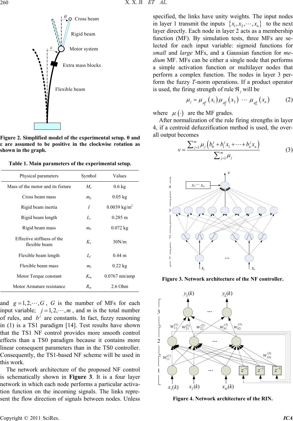

,

X. X. JI ET AL. 260
Rigid beam
Flexible beam
Motor system
Extra mass blocks
e
? Cross beam
θ
ε
Figure 2. Simplified model of the experimental setup. θ and
ε are assumed to be positive in the clockwise rotation as
shown in the graph.
Table 1. Main parameters of the experimental setup.
Physical parameters Symbol Values
Mass of the motor and its fixture Me 0.6 kg
Cross beam mass mp 0.05 kg
Rigid beam inertia I 0.0039 kg/m2
Rigid beam length Lr 0.285 m
Rigid beam mass mb 0.072 kg
Effective stiffness of the
flexible beam Ke 30N/m
Flexible beam length Lf 0.44 m
Flexible beam mass mf 0.22 kg
Motor Torque constant Km 0.0767 nm/amp
Motor Armature resistance Rm 2.6 Ohm
and 1, 2,,
g
G

, G is the number of MFs for each
input variable; , and m is the total number
of rules, and
1, 2,,jm
j
b are constants. In fact, fuzzy reasoning
in (1) is a TS1 paradigm [14]. Test results have shown
that the TS1 NF control provides more smooth control
effects than a TS0 paradigm because it contains more
linear consequent parameters than in the TS0 controller.
Consequently, the TS1-based NF scheme will be used in
this work.
The network architecture of the proposed NF control
is schematically shown in Figure 3. It is a four layer
network in which each node performs a particular activa-
tion function on the incoming signals. The links repre-
sent the flow direction of signals between nodes. Unless
specified, the links have unity weights. The input nodes
in layer 1 transmit the inputs

12
,,,
n

x
xx
j

to the next
layer directly. Each node in layer 2 acts as a membership
function (MF). By simulation tests, three MFs are se-
lected for each input variable: sigmoid functions for
small and large MFs, and a Gaussian function for me-
dium MF. MFs can be either a single node that performs
a simple activation function or multilayer nodes that
perform a complex function. The nodes in layer 3 per-
form the fuzzy T-norm operations. If a product operator
is used, the firing strength of rulewill be



12
12
gg g
n
j
n
A AA
x
x   x (2)
where





are the MF grades.
After normalization of the rule firing strengths in layer
4, if a centroid defuzzification method is used, the over-
all output becomes


011
1
1
mjj j
j
nn
j
m
j
j
bbxbx
v








(3)
4
v
1
x
? ? 
3
2
1
1
x? ? 
n
x
n
x
x
1
··· x
n
···
Figure 3. Network architecture of the NF controller.
1
z
L
y(k)
11
w
1
x(k)2
x(k)M x(k)
w11
(1 )
??
??
1
z1 z
(3)
N2
w(3)
NN
w(2)
1
y(k)
3
2
1
N1
w(3)
21
w(3 )
22
w(3)
??
···
···
···
Figure 4. Network architecture of the RIN.

X. X. JI ET AL.261
M
N
2
Once the NF control paradigm is established, its pa-
rameters should be trained properly so as to achieve op-
timal control performance. In this case, in each training
epoch, the nonlinear system parameters of the MFs are
trained by the gradient method in the backward pass,
whereas the linear consequent parameters are fine-tuned
by the LSE in the forward pass [14].
3. System Identification and Recurrent
Training (RT)
3.1. The Recurrent System Identification
Network
System identification is the process to recognize the
model of the tested plant automatically. One of the ad-
vantages of the intelligent control over the classical con-
trols is that system models can be identified by training
instead of analytical equations [15]. Real-time system
identification is especially important for the plants with
time-varying dynamics. In this work, a recurrent identi-
fication network (RIN) is developed to adaptively recog-
nize the system dynamics; its network architecture is
illustrated in Figure 4. It is a 3-layer network in which
each node performs a particular activation function on
the incoming signals. Layer 1 is the input layer. Layer 2
is the recurrent layer, in which each node has a weighted
feedback link to deal with time explicitly as opposed to
representing temporal information spatially. Each feed-
back unit copies the activation output of the correspond-
ing node from the previous time step for context proc-
essing; its purpose is to allow the network to memorize
cues from the past so as to improve modeling accuracy.
Let x(k) denote the M × 1 external input vector applied
to the RIN at the discrete time instant k, xi(k),
Assume that there are N recurrent neurons
in the hidden layer; Let denote the output of
the jth neuron in layer 2, . Then
is the forecasted output of the jth neuron
generated after one step at time step k + 1. The signal in
each feedback link represents the neuron output in the
previous time step (i.e., k – 1)
1, 2,,i


21
j
yk


2
j
yk
1, 2,,j


 



 222 1
11
1
NM
j
rjjij ij
ri
y
kwyk wxkb



 (4)
(1)
ij
w

i
is the weight of the link from the ith input
x
k in layer 1 to the jth neuron in layer 2; is
the weight of recurrent link from the rth neuron to the jth
neuron in layer 2;
(2)
rj
w
(2)
j
b is the bias of the jth neuron in
layer 2.
The network outputs

l
y
k in layer 3 are computed
as the summation of incoming signals:
 
(3) (2)
1
N
ljlj
j
ykwy k

 (5)
where l is the number of network outputs, 1, 2,,lL

;
(3)
j
l
w
1,
is the link weight between layer 2 and layer 3,
2, ,jN


3.2. Recurrent Training (RT) Technique
The RIN parameters should be tuned properly to improve
the adaptive capability of the controller to accommodate
different system conditions. Most of the currently used
system identification networks are trained by the classi-
cal training methods such as gradient algorithm and LSE
[15]. A novel training technique, recurrent training (RT),
will be suggested to fine-tune system parameters. Dif-
ferent from other real-time recurrent training, the pro-
posed RT technique can be used to optimize not only
recurrent links, but also the general feedforward links in
the recurrent NN. It aims to match the outputs of certain
neurons in a processing layer to their desired values at
specific time instants. The gradients in the RT technique
will be recursively computed at each time instant instead
of waiting until the end of the presented sequence as with
the general gradient-based algorithms. If the desired
(target) data sets are




,
dd
kk  , the objective func-
tion


O
Ek at time instant k will be defined as
 
2
1
1
2
L
Oldl
kl
EkEkykyk

  

 (6)
where


ld
y
k and


l
y
k are the lth desired output
and the corresponding RIN output from Equation (5),
respectively.
To minimize this objective function, we compute the
gradients of


(1) (2)
,
jww  
w
 
O
O
kk
jj
Ek
E
EEk


  

 ww
ww (7)
where


Ekw
)(k
is the gradient of the instantaneous
error with respect to the weights E
j

w.
In order to implement the proposed RT technique to
train the recurrent networks in real time, we will use an
instantaneous estimate of the gradient at time
step k. If

Ekw


(2)
j
yk is the output of the jth neuron in layer
2, the error-propagation at time instant k will be





 
 


(2)(2)
(2)
(2)(2) (2)
(2)
1
1
jj
jjj j
jjj
jj j
yk yk
Ek Ek
yk
ykykyk
yk















www
ww

(8)
To minimize


Ek, the gradients


j
Ek



w
in the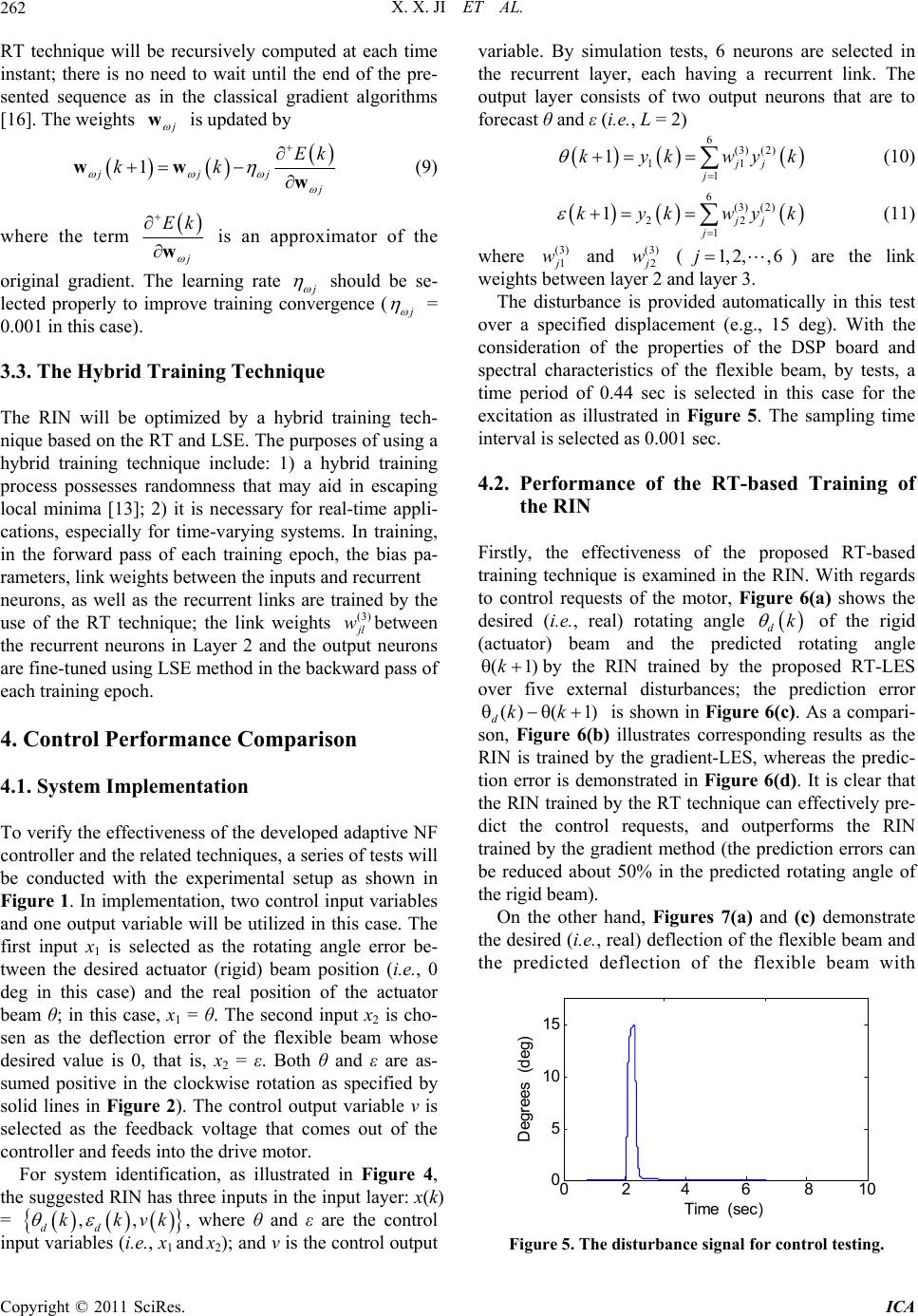

X. X. JI ET AL. 262
RT technique will be recursively computed at each time
instant; there is no need to wait until the end of the pre-
sented sequence as in the classical gradient algorithms
[16]. The weights
j

w is updated by
 
1
jjj
j
Ek
kk





 
ww w (9)
where the term

j
Ek



w is an approximator of the
original gradient. The learning rate
j


should be se-
lected properly to improve training convergence (
j


=
0.001 in this case).
3.3. The Hybrid Training Technique
The RIN will be optimized by a hybrid training tech-
nique based on the RT and LSE. The purposes of using a
hybrid training technique include: 1) a hybrid training
process possesses randomness that may aid in escaping
local minima [13]; 2) it is necessary for real-time appli-
cations, especially for time-varying systems. In training,
in the forward pass of each training epoch, the bias pa-
rameters, link weights between the inputs and recurrent
neurons, as well as the recurrent links are trained by the
use of the RT technique; the link weights between
the recurrent neurons in Layer 2 and the output neurons
are fine-tuned using LSE method in the backward pass of
each training epoch.
)3(
jl
w
4. Control Performance Comparison
4.1. System Implementation
To verify the effectiveness of the developed adaptive NF
controller and the related techniques, a series of tests will
be conducted with the experimental setup as shown in
Figure 1. In implementation, two control input variables
and one output variable will be utilized in this case. The
first input x1 is selected as the rotating angle error be-
tween the desired actuator (rigid) beam position (i.e., 0
deg in this case) and the real position of the actuator
beam θ; in this case, x1 = θ. The second input x2 is cho-
sen as the deflection error of the flexible beam whose
desired value is 0, that is, x2 = ε. Both θ and ε are as-
sumed positive in the clockwise rotation as specified by
solid lines in Figure 2). The control output variable v is
selected as the feedback voltage that comes out of the
controller and feeds into the drive motor.
For system identification, as illustrated in Figure 4,
the suggested RIN has three inputs in the input layer: x(k)
= , where θ and ε are the control
input variables (i.e., x1 and x2); and v is the control output
variable. By simulation tests, 6 neurons are selected in
the recurrent layer, each having a recurrent link. The
output layer consists of two output neurons that are to
forecast θ and ε (i.e., L = 2)
  
,,
dd
kkvk 


k
k
 
6(3) (2)
11
1
1jj
j
kykwy 

 
 (10)
 
6(3) (2)
22
1
1jj
j
kykwy 

 

(3)
(11)
where 1
j
w and 2
(3)
j
w () are the link
weights between layer 2 and layer 3.
1, 2,, 6j
The disturbance is provided automatically in this test
over a specified displacement (e.g., 15 deg). With the
consideration of the properties of the DSP board and
spectral characteristics of the flexible beam, by tests, a
time period of 0.44 sec is selected in this case for the
excitation as illustrated in Figure 5. The sampling time
interval is selected as 0.001 sec.
4.2. Performance of the RT-based Training of
the RIN
Firstly, the effectiveness of the proposed RT-based
training technique is examined in the RIN. With regards
to control requests of the motor, Figure 6(a) shows the
desired (i.e., real) rotating angle of the rigid
(actuator) beam and the predicted rotating angle

dk

)1(


k
)(
by the RIN trained by the proposed RT-LES
over five external disturbances; the prediction error
)1(




kk
d is shown in Figure 6(c). As a compari-
son, Figure 6(b) illustrates corresponding results as the
RIN is trained by the gradient-LES, whereas the predic-
tion error is demonstrated in Figure 6(d). It is clear that
the RIN trained by the RT technique can effectively pre-
dict the control requests, and outperforms the RIN
trained by the gradient method (the prediction errors can
be reduced about 50% in the predicted rotating angle of
the rigid beam).
On the other hand, Figures 7(a) and (c) demonstrate
the desired (i.e., real) deflection of the flexible beam and
the predicted deflection of the flexible beam with
04
0
5
10
15
Time (sec)
Degrees (deg)
10826
Figure 5. The disturbance signal for control testing.

X. X. JI ET AL.263
the RIN trained by the RT-LES and the gradient-LSE,
respectively. The corresponding prediction errors
are shown in Figures 7(c) and (d), re-
spectively. Apparently, the developed RIN can effec-
tively capture the plant’s dynamic behavior. The pro-
posed RT technique can significantly improve the per-
formance of system identification. The prediction error
)1()(  kk
d
01234
x 10
4
-10
0
10
20
Time Steps (ms)
Rotating Angle (degrees)
(a)
0 1 23 4
x 10
4
-10
-5
0
5
Errors (degree)
Time Steps (ms)
(b)
0 1 234
x 10
4
-10
0
10
20
Time Steps (ms)
Rotating Angle (degree)
(c)
0 1 23 4
x 10
4
-10
-5
0
5
Errors (degree)
Time Steps (ms)
(d)
Figure 6. Comparison of the desired (solid lines) and pre-
dicted (dotted lines) rotation of the rigid beam (control ef-
forts): (a) RIN is trained by RT-LSE, (b) error of rotating
angle; (c) RIN is trained by gradient-LSE; (d) error of ro-
tating angle.
01 2 3 4
x 10
4
-1
0
1
2
Deflection (cm)
Time Steps (ms)
(a)
01234
x 10
4
-1
-0.5
0
0.5
Errors (cm)
Time Steps (ms)
(b)
01234
x 10
4
-1
0
1
2
Deflection (cm)
Time Steps (ms)
(c)
01234
x 10
4
-1
-0.5
0
0. 5
Errors (cm)
Time Steps (ms)
(d)
Figure 7. Comparison of the desired (solid lines) and pre-
dicted (dotted lines) deflection of the flexible beam: (a) RIN
is trained by RT-LSE; (b) Error of deflection; (c) RIN is
trained by gradient-LSE; (d) Error of deflection.
of the deflection of the flexible beam can be reduced up
to 70% compared with the classical gradient algorithm.
4.3. Control Performance Comparison
To make a comparison, test results from the related NF
controllers with different scenarios will be listed:
1) Controller-1: using the same NF scheme as illus-
trated in Figure 3 without system identification. Its pur-

X. X. JI ET AL. 264
pose is to examine the efficiency of the system identifi-
cation process, especially for time-varying systems.
2) Controller-2: using the same NF control scheme;
but the system identification is based on a feedforward
NN which has the same number of network parameters
and is trained by the gradient algorithm.
3) Controller-3: using the same NF control scheme;
but the system identification is performed by the devel-
oped RIN which is trained by gradient-LSE method.
4) Controller-4: using the same NF control scheme;
but the system identification is performed by the devel-
oped RIN which is trained by the suggested RT-LSE
technique.
All the related controllers are implemented in MAT-
LAB Simulink. Firstly, we run the tests without extra
mass blocks attached. Figure 8 shows the control per-
formance of the related controllers over 10 seconds. It is
clear that the developed NF controller with the proposed
RIN and RT-based training (Controller-4) outperforms
other related controllers. The only difference between
Controller-1 and Controller-2 is related to the system
identification. A NF control without system identifica-
tion takes longer time to converge especially when the
beam is very flexible. A controller with efficient system
identification can facilitate the recognition of the plant’s
dynamics so as to improve control outperform. The dif-
ference between Controller-2 and Controller-3 is related
to the system identification strategy. It is clear that the
developed RIN can recognize the dynamics of the plant
more effectively and implement it for control operations.
The RIN outperforms the feedforward NN in system iden-
tification since the recurrent links in the RIN can store
context information so as to improve mapping between
0246810
-0. 5
0
0.5
1
Deflection (cm)
0246810
-0. 5
0
0.5
1
(a) (b)
(a) (b)
0246810
-0. 5
0
0.5
1
Time (sec)
Deflection (cm)
0246810
-0. 5
0
0.5
1
Time (sec)
(d) (c)
(c) (d)
Figure 8. Performance comparison without extra loads, by
(a) Controller-1, (b) Controller-2, (c) Controller-3, (d)
Controller-4.
the input space and the output space. The training con-
vergence of the NN control, however, is slow due to its
application of black box reasoning.
The only difference between Controller-3 and Con-
troller-4 is related to the suggested RT training (i.e.,
RT-LSE versus gradient-LSE). Compared with the clas-
sical gradient algorithm, the RT-related training can sig-
nificantly enhance training convergence and improve the
control performance. The training efficiency of the RT
technique is associated with its error-propagation which
is calculated at each time step instead of minimizing the
overall error function at the end of each sequence as in
gradient algorithm.
To verify the robustness of the developed controller
against time-varying conditions, a pair of adhesive mass
blocks is attached to the flexible beam in three different
locations during the tests: a top position about 5 cm be-
low the top end of the flexible beam, a middle position
(as shown in Figure 1), and a bottom position about 5
cm above the bottom end of the flexible beam. When the
mass blocks are attached to the beam, the dynamic prop-
erties of the plant (e.g., the mass distribution and natural
frequencies) will change, which will result in different
responses when a similar disturbance is applied to the
flexible beam. Figures 9-11 show the control perform-
ance comparison from different controllers as the extra
mass blocks are placed at three different positions of the
flexible beam. It is seen that the developed controller
(Controller-4) outperforms other controllers among these
control scenarios due to effective system identification
and training; Controller-4 is robust for time-varying con-
ditions. The proposed RT technique enables the control-
ler to effectively recognize and accommodate the new
0246810
-0. 5
0
0. 5
1
Deflection (cm)
02468 10
-0. 5
0
0.5
1
(a) (b)
(a) (b)
0246810
-0.5
0
0. 5
1
Time (sec)
De
f
lection
(
cm
)
0246810
-0.5
0
0. 5
1
Time (sec)
(d)
(c)
(c) (d)
Figure 9. Performance comparison when extra mass blocks
are placed at a top position of the flexible beam: by (a)
Controller-1, (b) Controller-2, (c) Controller-3, and (d)
Controller-4.

X. X. JI ET AL.265
0 2 4 6 810
-0. 5
0
0.5
1
Deflection (cm)
0 2 4 6 810
-0. 5
0
0. 5
1
(a)(b)
(a) (b)
0 2 4 6 810
-0. 5
0
0.5
1
Time (sec)
Deflection (cm)
0 2 4 6 810
-0. 5
0
0.5
1
Time (sec)
(d)(c)
(c) (d)
Figure 10. Performance comparison when extra mass
blocks are placed in a middle position of the flexible beam:
by (a) Controller-1, (b) Controller-2, (c) Controller-3, and
(d) Controller-4.
0 2 4 6 810
-0.5
0
0.5
1
Deflection (cm)
0 2 4 6 810
-0.5
0
0.5
1
(a) (b)
(a) (b)
0 2 4 6 810
-0.5
0
0.5
1
Time (sec)
Deflection (cm)
0 2 4 6 810
-0.5
0
0.5
1
Time (sec)
(d)
(d)
(c) (d)
Figure 11. Performance comparison when extra mass blocks
are placed at a bottom position of the flexible beam: by (a)
Controller-1, (b) Controller-2, (c) Controller-3, and (d)
Controller-4.
system dynamics. Furthermore, the hybrid training tech-
nique (e.g., RT-LSE) can reduce the sensitivity to the
initial conditions of the related parameters and improve
training convergence by reducing the possible trapping
due to local minima during the training process.
Controller-2 trained by the gradient method performs
reasonably well in these tests although it is prone to be-
ing trapped by local minima. The main reason is related
to the gradient-based searching algorithm.
It is seen that as extra masses are placed at different
positions of the flexible beam, there is no apparent con-
trol performance difference in terms of the overshoot,
undershoot, and settling time. It means that the NF para-
digm is a universal approximation [13] which contains
some adaptive capability to accommodate variance of
system dynamics. On the other hand, the RIN can more
effectively recognize new system dynamic conditions
and perform vibration suppression operations.
5. Conclusions
A novel NF controller is developed in this paper for ac-
tive vibration suppression in flexible structures. A novel
recurrent network, RIN, has been adopted to identify
system dynamics in real-time. A new RT-based hybrid
training technique is suggested to improve the conver
gence of the RIN scheme. The effectiveness of the de-
veloped NF controller and the related techniques has
been verified by experimental tests on the developed
experimental setup. The comprehensive test investigation
has demonstrated that the developed NF controller is an
effective strategy for active vibration suppression. The
RIN scheme can effectively recognize system dynamic
properties for real-time control operations. The RT-based
training technique can enhance convergence of training
and improve adaptive capability of the controller to ac-
commodate time-varying dynamics of the plants. The
developed NF controller is robust and outperforms other
related NF paradigms in terms of the control requests,
overshoot, undershoot, and settling time.
6. References
[1] D. Younesian, E. Esmailzadeh and R. Sedaghati, “Passive
Vibration Control of Beams Subjected to Random Exci-
tations with Peaked PSD,” Journal of Vibration and Con-
trol, Vol. 12, No. 9, 2006, pp. 941-953.
doi:10.1177/1077546306068060
[2] G. Genta, “Vibration Dynamics and Control,” Springer,
New York, 2009. doi:10.1007/978-0-387-79580-5
[3] Z. Mohamed, J. Martins, M. Tokhi, J. Costa and M. Botto,
“Vibration Control of a Very Flexible Manipulator Sys-
tem,” Control Engineering Practice, Vol. 13, No. 3, 2005,
pp. 267-277. doi:10.1007/978-0-387-79580-5
[4] K. Melhem and W. Wang, “Global Output Tracking Con-
trol of Flexible Joint Robots via Factorization of the Mass
Matrix,” IEEE Transactions on Robotics, Vol. 25, No. 2,
2009, pp. 248-257. doi:10.1007/978-0-387-79580-5
[5] M. Ishikawa, Y. Minami and T. Sugie, “Development and
Control Experiment of the Trident Snake Robot,” IEEE/
ASME Transactions on Mechatronics, Vol. 15, No. 1,
2010, pp. 9-16. doi:10.1109/TMECH.2008.2011985
[6] R. Jamil, “Inverse Dynamics Based Tuning of a Fuzzy
Logic Controller for a Single-Link Flexible Manipulator,”
Journal of Vibration and Control, Vol. 13, No. 12, 2007,
pp. 1741-1759. doi:10.1177/1077546307076282

X. X. JI ET AL. 266
[7] T. Li and S. Tsai, “T-S Fuzzy Bilinear Model and Fuzzy
Controller Design for a Class of Nonlinear Systems,”
IEEE Transactions on Fuzzy Systems, Vol. 15, No. 3,
2007, pp. 494-506. doi:10.1109/TFUZZ.2006.889964
[8] C. Ting, “An Observer-Based Approach to Controlling
Time-Delay Chaotic Systems via Takagi-Sugeno Fuzzy
Model,” Information Sciences, Vol. 177, No. 20, 2007, pp.
4314-4328. doi:10.1109/TFUZZ.2006.889964
[9] L. Tian and C. Collins, “A Dynamic Recurrent Neural
Network-Based Controller for a Rigid-Flexible Manipu-
lator System,” Mechatronics, Vol. 14, No. 5, 2004, pp.
471-490. doi:10.1109/TFUZZ.2006.889964
[10] M. Caswara and H. Unbehauen, “A Neurofuzzy Ap-
proach to the Control of a Flexible-Link Manipulator,”
IEEE Transaction on Robotics and Automation, Vol. 18,
No. 6, 2002, pp. 932-944. doi:10.1109/TRA.2002.805660
[11] L. Tian and C. Collins, “Adaptive Neuro-Fuzzy Control
of a Flexible Manipulator,” Mechatronics, Vol. 15, No.
10, 2005, pp. 1305-1320.
doi:10.1016/j.mechatronics.2005.02.001
[12] W. Wang and O. Jianu, “A Smart Monitor for Machinery
Fault Detection,” IEEE/ASME Transactions on Mecha-
tronics, Vol. 15, No. 1, 2010, pp. 70-78.
doi:10.1109/TMECH.2009.2016956
[13] W. Wang, “An Intelligent System for Machinery Condi-
tion Monitoring,” IEEE Transactions on Fuzzy Systems,
Vol. 16, No. 1, 2008, pp. 110-122.
doi:10.1109/TFUZZ.2007.896237
[14] Z. Sun, K. Au and T. Choi, “A Neuro-Fuzzy Inference
System through Integration of Fuzzy Logic and Extreme
Learning Machines,” IEEE Transactions on Systems,
Man, and Cybernetics-Part B: Cybernetics, Vol. 37, No.
5, 2007, pp. 1321-1331.
doi:10.1109/TSMCB.2007.901375
[15] P. Mastorocostas and J. Theocharis, “A Recurrent
Fuzzy-Neural Model for Dynamic System Identification,”
IEEE Transactions on System, Man and Cybernetics-Part
B: Cybernetics, Vol. 32, No. 2, 2002, pp. 176-190.
[16] K. Christodoulou and C. Papadimitriou, “Structural Iden-
tification Based on Optimally Weighted Modal Residu-
als,” Mechanical System and Signal Processing, Vol. 21,
No. 1, 2007, pp. 4-23. doi:10.1016/j.ymssp.2006.05.011