Intelligent Control and Automation, 2011, 2, 167-175
doi:10.4236/ica.2011.23020 Published Online August 2011 (http://www.SciRP.org/journal/ica)
Neural Modeling of Multivariable Nonlinear Stochastic
System. Va riable Learning Rate Case
Ayachi Errachdi, Ihsen Saad, Mohamed Benrejeb
Unit of Research LARA Automatic, le Belvedere, Tunisia
Received December 23, 2010; revised January 20, 2011; accepted January 27, 2011
Abstract
The objective of this paper is to develop a variable learning rate for neural modeling of multivariable
nonlinear stochastic system. The corresponding parameter is obtained by gradient descent method optimiza-
tion. The effectiveness of the suggested algorithm applied to the identification of behavior of two nonlinear
stochastic systems is demonstrated by simulation experiments.
Keywords: Neural Networks, Multivariable System, Stochastic, Learning Rate, Modeling
1. Introduction
The Neural Networks (NN) was well used in modeling of
nonlinear systems because of its ability of learning, its
generalization and its approximation [1-4]. Indeed, this
approach provides an effective solution for wide classes
of nonlinear systems which are not known or only partial
state information is available [5].
Identification is the process of determining the dy-
namic model of a system from measurements inputs/
outputs [6]. Often, the measured output system is tainted
noise. This is due either to the effect of disturbances act-
ing at different parts of the process, either to measure-
ment noise. Therefore these noises may introduce errors
in the identification. The stochastic model is a solution to
overcome this problem [7]. In this paper, a multivariable
nonlinear stochastic system is our interest.
Among the parameters of the NN model, the learning
rate ()

has an important role in training phase. In this
phase several tests are taken account to find the suitable
fixed value. For instance, this parameter can slow down
this phase of training [8,9] if it is small. However, if this
parameter is large, the training phase is occurring quickly
and it becomes unstable [8,9]. To overcome this problem,
an adaptive learning rate was asked in [8,9]. This solu-
tion is applied in training algorithm of a nonlinear sin-
gle-variable system [8] and in multivariable nonlinear
system [9]. In this paper, a variable learning rate of neu-
ral network is developed in order to model a multivari-
able nonlinear stochastic system. Different cases of sig-
nal ratio to noise (SNR) are taken account to show the
influence of the noise in identification and the stability of
training phase.
This paper is organized as follows. In second section,
a multivariable system modeling by neural networks is
presented. In third section, the fixed learning rate method
is showed. The simulation of the multivariable stochastic
systems by NN method using fixed learning rate is de-
tailed in the fourth section. The development of the
variable learning rate and results simulations are pre-
sented in fifth section. Conclusions are given in sixth
section.
2. Multivariable System Modeling by Neural
Networks
To find the neural model of such nonlinear systems,
some stages must be respected [10]. Firstly the input
variables are standardized and centered. Then, the struc-
ture of the model is chosen. Finally, the synaptic weights
are estimated and the obtained model must be validated.
In this context, different algorithms are interested of the
synaptic weights estimation. For instance, the gradient
descent algorithm [11], the conjugate gradient algorithm
[11], the one step secant [11], the Levenberg-Marquardt
method [11] and resilient Backpropagation algorithm [11]
are developed and confirmed their effectiveness in train-
ing. In this paper, the gradient descent algorithm is our
interest.
On the basis of the input and output relation of a sys-
tem, the above nonlinear system can be expressed by a
NARMA (Nonlinear Auto-Regressive Moving Average)

A. ERRACHDI ET AL. 168
1,
N
il
model [12], that is given by the Equation (1). The archi-
tecture of the RNN is presented in Figure 1.
 
 
2
1
1,,
,,1
ipii
ii
ykfykyk n
uk ukn
  

 


 (1)
The output of the hidden node is given by the
following equation:
th
l
1
2
1
,1,,
N
lljj
j
hpvl


 (2)
The neural output is given by the following equa-
tion:
th
i


21
2
11
1
1
, 1,,
NN
iljj
lj
N
lil
l
okffpv z
f
fhz ins






 













1





(3)
Finally, the compact form is defined as:







 
2
22
2
1
111 1
1
1
1
1
1
...
ns
Nns
NnsN
N
T
ok
Ok
ok
fhfh zz
f
zz
fh fh
fZ kFPkvk
































 


(4)
where





1
2211
2
11 1
1
1
...
N
NNNN
N
T
pp
fh vk
f
ppvk
fh
FPv


 


 
 
 


 
 






The principle of neural modeling of the multivariable
stochastic system is showing in Figure 1.
To show the influence of disturbances on modeling, a
noise signal is added to the output system. Dif-
ferent cases of Signal Noise Ratio (i SNR ) are taken. This
(i SNR ) measures the correspondence between the system
output and the estimated output, the equation of
is as follows:

i
bk
i
SNR


 
0
0
1
1
N
ii
k
iN
ii
k
yk y
N
SNR bkb
N







(5)
u
nu
(k)
-
+
-
+
e
ns
(k+1)
e
1
(k+1)
o
ns
(k+1)
o1
(k+1)
y
ns
(k+1)
y
1
(k+1)
Disturbances
u
1
(k)
On-line
Learning
z
v p
Process
TDL
TDL
TDL
TDL
Figure 1. Principle of the neural modeling of the multivari-
able stochastic system.
The accuracy of correlations relative to the measured
values is finding by various statistical means. The criteria
exploited in this study were the Relative Error (RE),
Root Mean Square Error (RMSE) and Mean Absolute
Percentage Error (MAPE) [11] given by :



12
22
ii i
RE Eyoy






 (6)
  
0
100 N
ii
ki
M
APE eykok
N

 (7)
3. Fixed Learning Rate Method
The neural system modeling is the research of parame-
ters (weights) model. The search of these weights is the
subjects of different works [1-6,8-13]. The gradient de-
scent method is one among different methods which was
well applied on neural identification for single-variable
system [8] and for multivariable system [9]. In this paper,
the same principle is suggested to be applied on neural
identification of the multivariable stochastic systems.
Indeed, the criterion is minimized as follows:
th
i
    
22
11
22
ii ii
J
kek ykok

(8)
By application of the GD method, the theory of [1] is
used; we find then [9]:
 For the variation of the synaptic weights of the hidden
layer towards the output layer with s.

1, ,in


   
ii
il iii
il il
Jk ok
ze
zk zk


 

k (9)
The compact form (4) is used here, so we find



 
 
'
T
il
ilili
il
il i
zFPv
zfh e
zk
fhFPvek




 

k
(10)

A. ERRACHDI ET AL.169
Finally, the synaptic weights of the hidden layer to-
wards the output layer can be written in the following
way:
   
1
ilili li
zk zkfhFPvek 

 (11)
 For the variation of the synaptic weights of the input
layer towards the hidden layer.



 



 
  
i
lji lj
i
ii
lj
T
il
il i
lj
T
il ili
Jk
ppk
okek
pk
zFPv
f
he
pk k
f
hFPvzvek












 
(12)
Finally, the synaptic weights of input layer towards the
hidden layer can be written in the following way:
   


1
ljlji lili
pk pkfhFPvzkek 
  (13)
In these expressions, i

is a positive constant value
[8,9] which represents the learning rate (0 1)
i

 and

F
Pv
 represents Jacobian matrix of

F
Pv
T
.

1
1,, 2
1lN
N
lj j
j
FPv diagfpv












(14)
1
1
1
2
1
1
11, ,
N
lj j
Nj
lj jN
j
lj j
jlN
fpv
fpv
pv
















(15)
4. Simulation of Multivariable Nonlinear
Stochastic System s (5)SNR 

In this section, two types of multivariable nonlinear sto-
chastic systems with 2 dimensions are
presented with . The system

[8] and
[14] are defined respectively by the following
equations:

2, 2nu ns

1
S

5SNR 

2
S




 
 
  
 



111
1
1
111
222
2
12
10.30.6 1
0.6sinπ
+0.3sin3π
0.1sin5π
10.30.6 1
0.8sin2
1.2
ykykyk
uk
uk
Suk bk
ykyk yk
yk
uk bk
 






 












 



11
32
2
12
2
1
2
112 1
22
2
2
0.8
12
0.8
12
yk ukuk
yk yk
bk
Syk ykykuk
yk yk
bk













(17)
with 1 and 2 are a random signals, or 1 u and 2
are the input signals of the systems considered defined
by:
b bu

1
2π
sin 250
k
uk  



(18)
and

2
2π
sin 25
k
uk  



(19)
The input signal and are presented in Figure
2.
1
u2 u
4.1. Simulation Results of System (S1)
A dynamic NN is used to simulate a multivariable
nonlinear stochastic system (S1)

. In Figure
3, the evolution of the process output and the NN output
of the system (S1) is presented. The estimation error be-
tween these two outputs is presented in Figure 4.

5SNR 
The obtained results, present that for a fixed learning
rate 10.32


, the NN output 1 follows the measured
output 1 with an error of prediction and
that 2 follows the measured output 2 with an error
of prediction
o
y
oe
10.0720e
y
20.0601

whose learning rate is
20.27


.
0500 1000
-1
-0.5
0
0.5
1
input signal : u
1
k
0500 1000
-1
0
1
input signal :u
2
k


(16)
Figure 2. Input signals of the multivariable nonlinear sto-
chastic system.

A. ERRACHDI ET AL. 170
0200 400 600800 1000
-8
-6
-4
-2
0
k
P roc es s Out put (r) : y
1
& N N (b) : o
1
0200 400600 800 1000
-8
-6
-4
-2
0
P roc e s s Output (r) : y2 & NN (b) : o
2
k
Figure 3. Output of process and NN of system (S1) using a
fixed learning rate.
0200 400 600 8001000
-0.1
0
0.1
Learning E rror :e1
k
0200 400 600 8001000
-0.1
0
0.1
Learning E rror :e
2
k
Figure 4. Learning error between the output of process and
NN.
If this system has not an added noise, the error of pre-
diction is and
10.0384e20.0375e

[9].
4.2. Simulation Results of System (S2)
A dynamic NN is used to simulate a multivariable
nonlinear stochastic system (S2)

. In Figure
5, the evolution of the process output and the NN output
of the system (S2) is presented. The estimation error be-
tween these two outputs is presented in Figure 6.

5SNR 
The obtained results showing in Figure 5, present that
for a fixed learning rate 10.3


, the NN output 1 o
follows the measured output 1 with an error of predic-
tion 1 and that 2
o follows the meas- ured
output with an error of prediction
y
0.0650e
2
y20.06e70

0500 1000
-8
-6
-4
-2
0
P roces s Output (r) : y
1
& NN (b) : o
1
k
0500 1000
-8
-6
-4
-2
0
P rocess Output (r) : y2 & NN (b) : o2
k
Figure 5. Output of process and NN of system (S2) using
fixed learning rate.
0500 1000
-0.1
0
0.1
Learning E rror : e
1
k
0500 1000
-0.1
0
0. 1
Learni ng Err or : e2
k
Figure 6. Learning error between the output of process and
NN.
whose learning rate is 20.25


.
However, if 10b

and , the error of predict-
tion is
20b
10.0531e

2
Table 1 shows the obtained results of each statistical
indicator in the system (S1) and (S2) in the case of fixed
learning rate.
and [9].
0.0471e
Three cases of


SNR5,10 and 20 are taken to show
the influence of disturbances modeling. The obtained
results are presented in Table 2 for the first system and
in table 3 for the second system.
In both Tables 2 and 3, when the increases the
SNR


i
mse e decrease, it is due under the presence of dis-
turbances in the system.
In this section, the simulation of the two systems (S1
and S2) is carried out using a fixed learning rate. To find

A. ERRACHDI ET AL.171
Table 1. Values of different statistical indicators.
SNR = 5% RE MAPE
S1
S2
e1
e2
e1
e2
4.370e – 4
4.106e – 4
2.616e – 4
3.542e – 4
0.0437
0.0211
0.0262
0.0354
Table 2. Different cases of SNR.
SNR 5% 10% 20%
mse(e1) 7.611e – 5 6.679e – 5 5.648e – 5
mse(e2) 7.458e – 5 6.643e – 5 4.205e – 5
Table 3. Different cases of SNR.
SNR 5% 10% 20%
mse(e1) 8.698e – 5 7.705e – 5 5.947e – 5
mse(e2) 8.688e – 5 7.562e – 5 5.278e – 5
the suitable learning rate it is necessary to carry out sev-
eral tests by keeping the condition that . This
research of the learning rate can slow down the phase of
training. To cure this disadvantage and in order to accel-
erate the phase of training, a variable learning rate is used
and a fast algorithm will be developed.

0
i
 1
)
5. The Proposed Fast Algorithm
The need for using a variable learning rate is to have a
fast training [8-9,15-18]. To answer this condition, the
difference of the estimation error at and at
is calculated [8,9].
th
i(1k

k



 
11
iiii
ii
ek ekyk ok
yk ok



1
(20)
We suppose that




11
and
11
ii
iii
ykyk yk
okokok
 
 


i
(21)
by application of [8,9]
 
1
ii
yk ok 1
(22)
then the Equation (20) can be




 

  
11
ii i
i
ii l
lj
TT
lilil
ek ekok
okek fh
pk
We introduce (10) and (12),




   
   
1
+
ii
T
lil
TT
ililili
ek ek
i
f
hFPv fhFPvek
zFPvfhF Pvzvekv




 
  
(24)
so we find



  



 
22
1
T
iiil
TT
ilil i
ii i
ekekfhFPvFPv
zF PvF Pvzvvek
ke k


 
 
 


(25)
with



 

22
il
T
il
T
il
kfhFPvFP
zF PvF Pvzvv

 

 


T
v
(26)
at


1k

the estimation error is
th
i


11
iii
ekk ek    


i
(27)
To ensure the convergence of the estimation error,
th
i
i.e.,


lim 0
i
kek 

, the condition

11
ii k
  has to
be satisfied [8,9]. This condition implies


1
02
ii
k 


i
. It is clear that the upper range of the
learning rate (

) is variable because


ik
 depends on
, il and lj. The fastest learning occurs when the
learning rate is:
vzp
 



122
() 1'
''
il
T
ii l
TT
il
kfhFPvF
zF PvF Pvzvv
 

 


Pv
(28)
Note that this selection of i

implies






11 0ekk ek 
iiii

 

. It’s certain that the
learning process cannot finish instantly because of the
approximation which is caused by the finite sampling
time contrary to the theory which is proved that it can be
happen if infinitely fast sampling can occur.
lj
f
hFPvzzFPvPv


 




 
 
(23)
Using the obtained variable learning rate i

, the syn-
aptic weights il z

and lj p

will be respectively. it’s
certain that the learning process cannot finish instantly
because of the approximation caused by the finite sam-
pling time contrary to the theorie which proved that it
can be happen if infinitely fast sampling can occur it’s
certain that the learning process cannot finish instantly
because of the approximation caused by the finite sam-
pling time contrary to the theorie which proved that it
can be happen if infinitely fast sampling can occur it’s
certain that the learning process cannot finish instantly
because of the approximation caused by the finite sam-
pling time contrary to the theorie which proved that it
can be happen if infinitely fast sampling can occur it’s

A. ERRACHDI ET AL. 172
certain that the learning process cannot finish instantly
because of the approximation caused by the finite sam-
pling time contrary to the theorie which proved that it
can be happen if infinitely fast sampling can occur.






  
i
il iliTT
lil
FPvek
zfhFPvek T
il
f
hFPv FPvzFPv FPvzvv
 

 





(29)
  


  
()
il i T
ljilil iTT
lil
FPvzvek
pfhFPvzvek T
T
il
f
hFPvFPvzFPvFPvzvv
 


 

 



(30)
Finally, and can be:

il
zk lj p
 




 
1()
i
il ilTT
lil
FPvek
zk zkT
il
f
hFPvFPvzFPvFPvzvv 






(31)
 




  
1il i
lj ljTT
lil
FPvzvek
pk pkT
T
il
f
hFPvFPvzFPvF Pvzvv 



 



(32)
rate, the neural output 1 follows the measured output
1 with an error of prediction 1 and that 2
follows the measured output 2 with an error of predict-
tion 2
o
y0.0634eo
y
0.0588e

. However, if and
10b20b

, the
error of prediction is 10.0175e

and [9].
2
e0.0369
5.1. Simulation Results of System (S1)
(5)SNR 
In this section, the obtained variable learning rate (1

,2

)
are applied. In Figure 7, the evolution of the process
output and the NN output of the system (S1) is presented.
The error estimation between these two outputs is pre-
sented in Figure 8.
5.2. Simulation Results of System (S2)
(5)SNR

The obtained results present that for a variable learning
The evolution of the process output and the NN output of
the system (S2) is presented in Figure 9. The error be-
tween these two outputs is presented in Figure 10. The
evolution of the squared error in two cases; fixed and
variable learning rates is presented in Figures 11 and 12.
0200400600800 1000
-8
-6
-4
-2
0
Process Output (r) : y
1
& NN (b) : o
1
k
0200 400 600 800 1000
-8
-6
-4
-2
0
P rocess O ut put (r) : y
2
& NN (b) : o
2
k
The obtained results, concerning system (S2), present
that for a variable learning rate, the neural output 1
follows the measured output with an error of pre-
dicttion
o
1
y
10.0539e

and that 2 follows the measured
output with an error of prediction
o
2
y20.06e68

.
0200 400 600 8001000
-0.1
0
0.1
Learning E rror :e
1
k
0200 400600 800 1000
-0.1
0
0.1
Learning Error :e
2
k
Figure 7. Output of process and NN of system (S1) using a
variable learning rate. Figure 8. Learning error between the output of process and
NN.

A. ERRACHDI ET AL.173
0200 400 600 800 1000
-8
-6
-4
-2
0
Proces s Output (r) : y
1
& NN (b) : o
1
k
0200 400 600800 1000
-8
-6
-4
-2
0
Proces s Output (r) : y
2
& NN (b) : o
2
k
Figure 9. Output of process and NN of system (S2) using a
variable learning rate.
0200 400600 8001000
-0.1
0
0.1
Learning Error :e
1
k
0200 400 600800 1000
-0.1
0
0.1
Learning Error :e
2
k
Figure 10. Learning error between the output of process
and NN.
However, if and , the error of prediction
is and [9].
10b
2
20b
0.0166
1 2
The obtained results presented in Figures 11 and 12
showing that, when a variable learning rate is used, the
convergence of the squared error is very faster than a
fixed learning rate is used.
0.029ee
Table 4 shows the obtained results of each statistical
indicator in the system (S1) and (S2) in the case of vari-
able learning rate.
We took three cases of to show
the influence of disturbances modeling. The obtained
results are presented in Table 5 for the first system and
in Table 6 for the second system. In both tables, when
the increases the decrease, it is due un-
der the presence of disturbances in the system.
(5,10 and 20)SNR
()
i
e eSNR ms
The obtained values in Tables 5 and 6 are
lower compared to which are calculated in Ta-
bles 2 and 3, that explains the variable rate adjusts with
()
i
mse e
()
i
e ems
0200 400 600 8001000
0
0.5
1x 10
-8
iterations
Mean Squer E rror
Fixed rate:0.32
V ariabl e rat e
0200 400 600 8001000
0
2
4
6
8x 10
-4
iterations
Mean Sq uer Error
fixed rate:0.27
V a ri abl e rate
Figure 11. Evolution of the mean squared error of (S1).
0200 400 600 8001000
0
1
2
3x 10
-9
iterati ons
Mean Squer Err or
Fixed rate:0.3
V ariable rat e
0200 400600800 1000
0
2
4
6
8x 10
-3
iterat ions
mean Squer Error
fixed rate:0.25
Variable rate
Figure 12. Evolution of the mean squared error of (S2).
Table 4. Values of different statistical indicators.
SNR = 5% RE MAPE
S1
S2
e1
e2
e1
e2
3.256e – 4
3.793e – 4
6.453e – 4
6.236e – 4
0.0326
0.0379
0.0645
0.0624
Table 5. Different cases of SNR.
SNR 5% 10% 20%
mse(e1)
mse(e2)
5.906e – 5
6.501e – 5
5.152e – 5
5.552e – 5
3.932e – 5
4.310e – 5
Table 6. Different cases of SNR.
SNR 5% 10% 20%
mse(e1)
mse(e2)
7.402e – 5
7.863e – 5
6.368e – 5
4.601e – 5
6.334e – 5
4.537e – 5

A. ERRACHDI ET AL. 174
changes in examples.
6. Conclusions
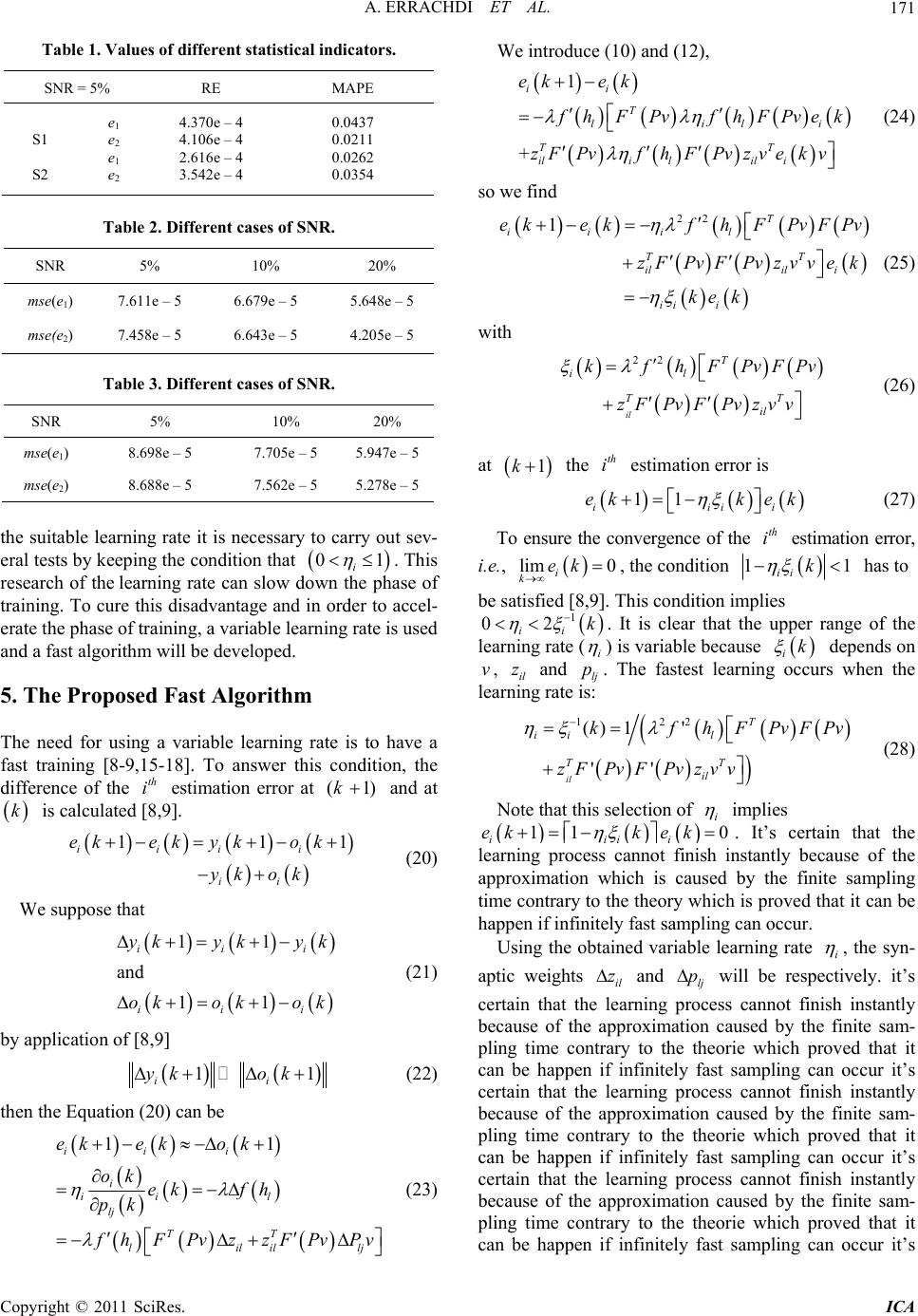
In this paper, a variable learning rate for neural modeling
of multivariable nonlinear stochastic system is suggested.
This parameter can slow down the training phase when it
is chosen as small, and can be unstable when it is chosen
as large. To avoid this step, a variable learning rate
method is developed and it is applied in identification of
nonlinear stochastic system. The advantages of the pro-
posed algorithm are firstly the simplicity to apply it in a
multi-input multi-output nonlinear system. Secondly, the
gain of the training time is remarked and the result qual-
ity is noticed. Besides, this algorithm is a manner to
avoid the search for such fixed training rate which pre-
sents a disadvantage at the level the phase of training. In
contrary, the variable learning rate algorithm does not
require any experimentation for the selection of an ap-
propriate value of the learning rate. The proposed algo-
rithm can be applied in real time process modeling. Dif-
ferent cases of SNR are discussed to test the developed
method and it showed that the obtained results using a
variable learning rate is very satisfy than when the fixed
learning rate was used.
7. References
[1] K. Kara, “Application des Réseaux de Neurones à
l’identification des Systèmes Non Linéaire,” Thesis, Con-
stantine University, 1995.
[2] S. R. Chu, R. Shoureshi and N. Tenorio “Neural Net-
works for System Identification,” IEEE Control System
Magazine, Vol. 10, No. 3, 1990, pp. 31-35.
[3] S. Chen and S. A. Billings, “Neural Networks for Non-
linear System Modeling and Identification,” Inernational
Journal of Control, Vol. 56, No. 2, 1992, pp. 319-346.
doi:10.1080/00207179208934317
[4] N. N. Karabutov, “Structures, Fields and Methods of
Iden- tification of Nonlinear Static Systems in the Condi-
tions of Uncertainty,” Intelligent Control and Automation
(ICA), Vol. 1, No. 1, 2010, pp. 1-59.
[5] D. C. Psichogios and L. H. Ungar, “Direct and Indirect
Model-Based Control Using Artificial Neural Networks,”
Industrial and Engineering Chemistry Research, Vol. 30,
No. 12, 1991, pp. 25-64.
doi:10.1021/ie00060a009
[6] A. Errachdi, I. Saad and M. Benrejeb, “On-Line Identify-
cation Method Based on Dynamic Neural Network,” In-
ternational Review of Automatic Control, Vol. 3, No. 5,
2010, pp. 474-479.
[7] A. M. Subramaniam, A. Manju and M. J. Nigam, “A
Novel Stochastic Algorithm Using Pythagorean Means
for Minimization,” Intelligent Control and Automation,
Vol. 1, No. 1, 2010, pp. 82-89.
doi:10.4236/ica.2010.12009
[8] D. Sha and B. Bajic, “On-Line Adaptive Learning Rate
BP Algorithm for MLP and Application to an Identifica-
tion Problem,” Journal of Applied Computer Science, Vol.
7, No. 2, 1999, pp. 67-82.
[9] A. Errachdi, I. Saad and M. Benrejeb, “Neural Modelling
of Multivariable Nonlinear System. Variable Learning
Rate Case,” 18th Mediterranean Conference on Control
and Automation, Marrakech, 2010, pp. 557-562.
[10] P. Borne, M. Benrejeb and J. Haggege, “Les Réseaux de
Neurones. Présentation et Application,” Editions Technip,
Paris, 2007.
[11] S. Chabaa, A. Zeroual and J. Antari, “Identification and
Prediction of Internet Traffic Using Artificial Neural Net-
Works,” Journal of Intelligent Learning Systems & Ap-
plications, Vol. 2, No. 1, 2010, pp. 147-155.
[12] M. Korenberg, S. A. Billings, Y. P. Liu and P. J. Mcllroy,
“Orthogonal Parameter Estimation Algorithm for Non-
linear Stochastic Systems,” International Journal of Con-
trol, Vol. 48, No. 1, 1988, pp. 346-354.
doi:10.1080/00207178808906169
[13] A. Errachdi, I. Saad and M. Benrejeb, “Internal Model
Control for Nonlinear Time-Varying System Using Neu-
ral Networks,” 11th International Conference on Sciences
and Techniques of Automatic Control & Computer Engi-
neering, Anaheim, 2010, pp. 1-13.
[14] D. Sha, “A New Neural Networks Based Adaptive Model
Predictive Control for Unknown Multiple Variable
No-Linear systems,” International Journal of Advanced
Mechatronic Systems, Vol. 1, No. 2, 2008, pp. 146-155.
doi:10.1504/IJAMECHS.2008.022013
[15] R. P. Brent, “Fast Training Algorithms for Multilayer
Neural Nets,” IEEE Transactions on Neural Networks,
Vol. 2, No. 3, 1991, pp. 346-354.
doi:10.1109/72.97911
[16] R. A. Jacobs, “Increase Rates of Convergence through
Learning Rate Adaptation,” IEEE Transactions on Neural
Networks, Vol. 1, No. 4, 1988, pp. 295-307.
[17] D. C. Park, M. A. El-Sharkawi and R. J. Marks, “An
Adaptively Trained Neural Network,” IEEE Transactions
on Neural Networks, Vol. 2, No. 3, 1991, pp. 334-345.
doi:10.1109/72.97910
[18] P. Saratchandran, “Dynamic Programming Approach to
Optimal Weight Selection in Multilayer Neural Net-
works,” IEEE Transactions on Neural Networks, Vol. 2,
No. 4, 1991, pp. 465-467. doi:10.1109/72.88167

A. ERRACHDI ET AL. 175
Nomenclature
i
y: vector of process output, its average valuei y,
i
u: vector of process input,
p
f
: unknown function of process,
1
n: input delay,
2
n: output delay, ,
12
nn
U: input of the process,
 
1
T
n
Uukuk




,
Y: output of the process,
 
1
T
ns
Yykyk




,
i
o: vector of RNN output,
O: output of the RNN model, ,

1
T
ns
Oo o
1
N: number of nodes of input layer,
2
N: number of nodes of hidden layer,
lj
p: synaptic weights of the input layer towards the hid-
den layer, lj
P
p   with and
,
2
1, ,lN
1
1, ,jN
v: input vector of the RNN model,


1
1
1
2
()(1)()
(1)
N
ii i
i
vvv
ukuk nyk
yk n







,
ns : number of nodes of output layer,
il
z: synaptic weights of hidden layer towards the output
layer,


il
Z
z with 2 1, ,lN

 and , 1,,ins
i

: learning rate, 01
i


,

: a scaling coefficient used to expand the range of
RNN output, 01


,
f
: activation function,


l
f
h is the output of the
node,
th
l


i
ek: error between the measured process output
and the measured RNN output,
th
i
th
i






i
ekk ok(
ii
y,
E: vector of error,
 
1
T
ns
Eekek




,
N: number of observations,
TDL: Tapped Delay Line block,
l
h: output of neuron of hidden layer,
th
l
 


2
1
T
N
FPvfh fh








1
FPv diagfhf
,

2
T
N
h






,


i
bk: noise of measurement of symmetric terminal

,




,,bk
i

  
i
b: noise average value.