J. Biomedical Science and Engineering, 2008, 1, 133-140
Published Online August 2008 in SciRes. http://www.srpublishing.org/journal/jbise JBiSE
Visualization of protein structure relationships us-
ing constrained twin kernel embedding
Yi Guo1, Jun-Bin Gao2, Paul Wing Hing Kwan1 & Kevin Xinsheng Hou3
1School of Science and Technology University of New England, Armidale, NSW 2351, Australia. 2School of Computer Science Charles Sturt University,
Bathurst, NSW 2795, Australia. 3School of Biological, Biomedical and Molecular Sciences University of New England, Armidale, NSW 2351, Australia.
Correspondence should be addressed to Yi Guo ([e-mail]), Jun-Bin Gao ([e-mail]), Paul W. Kwan ([e-mail]), and
Kevin X. H ou ( [e-mail]).
ABSTRACT
In this paper, a recently proposed dimensional-
ity reduction method called Twin Kernel Em-
bedding (TKE) [10] is applied in 2-dimensional
visualization of protein structure relationships.
By matching the similarity measures of the in-
put and the embedding spaces expressed by
their respective kernels, TKE ensures that both
local and global proximity information are pre-
served simultaneously. Experiments conducted
on a subset of the Structural Classification Of
Protein (SCOP) database confirmed the effec-
tiveness of TKE in preserving the original rela-
tionships among protein structures in the low er
dimensional embedding according to their simi-
larities. This result is expected to benefit sub-
sequent analyses of protein structures and their
functions.
1. INTRODUCTION
Recent years have seen phenomenal advances in dimen-
sionality reduction (DR) methods that are widely applied
in bioinformatics [26, 14, 6, 16], biometrics [19, 4, 15,
17], robotics [11], etc. The rapid growth of DR methods
stems from the need to reduce the complexity of the
problem at hand. The target of these methods is mainly
to find the corresponding counterparts of the input data
in a much lower dimensional space without incurring
significant information loss. The low dimensional repre-
sentation can be used in subsequent procedures such as
classification, pattern recognition, and so on. For exam-
ple, a medium sized protein structure typically has a few
thousands of degrees of freedom which is naturally re-
siding in very high dimensional space. It causes the so-
called “curse of dimensionality” problem which will not
only drastically increase the computational complexity of
the learning algorithms but also require large storage
space, leading to very slow indexing and searching speed
in a large scale database in the sequel. Through DR,
most of the redundant dimensions can be removed and
the degrees of freedom left are then input to the subse-
quent discriminant and classification tasks with consid-
erable simplication.
Another advantage of using DR is the 2- or 3-
dimensional mappings of the original data can be visual-
ized in an Euclidean space that can facilitate interpreting
the relationships among data by the researchers. Nor-
mally, the relationships among a set of protein structures
are typically represented in the form of trees derived by
hierarchical clustering. However, this representation
only provides some hints on the evolutionary distances
between protein structures. This limitation motivates our
applying to the application of DR methods in visualizing
the similarity relationships among protein structures.
In this paper, we will propose a new DR algorithm
called Constrained Twin Kernel Embedding (CTKE)
based on Twin Kernel Embedding (TKE) [10] to achieve
the above target. To provide the necessary background
knowledge, we will first give a brief review of DR meth-
ods on protein structures in the next section, followed by
an introduction of TKE and related topics involved in
this new algorithm. Then the CTKE algorithm will be
introduced, which integrates the similarity matching by
TKE with the objective function used in LS-SVM [23].
Experiments on real protein structure data will be pre-
sented and finally we summarize this paper with a con-
clusion.
2. THE RELATED WORKS
DR methods can be categorized into Linear DR methods
(LDR) such as Principal Component Analysis (PCA)
[13], Linear Discriminant Analysis (LDA) [7] and
NonLinear DR methods (NLDR) such as ISOMAP [25],
Laplacian Eigenmaps (LE) [3], Locally Linear Embed-
ding (LLE) [20], etc. LDR methods have been widely
used in bioinfo rmatics due to their simplicity. For exam-
ple, Teodoro et al. [27] applied PCA to transform the
original high dimensional protein motion data into a
lower dimensional representation th at captures the domi-
nant modes of motions of the protein. However, the line-
arity assumption on which linear methods are con-
structed does not hold in most cases. In [5], Das et al.
SciRes Copyright © 2008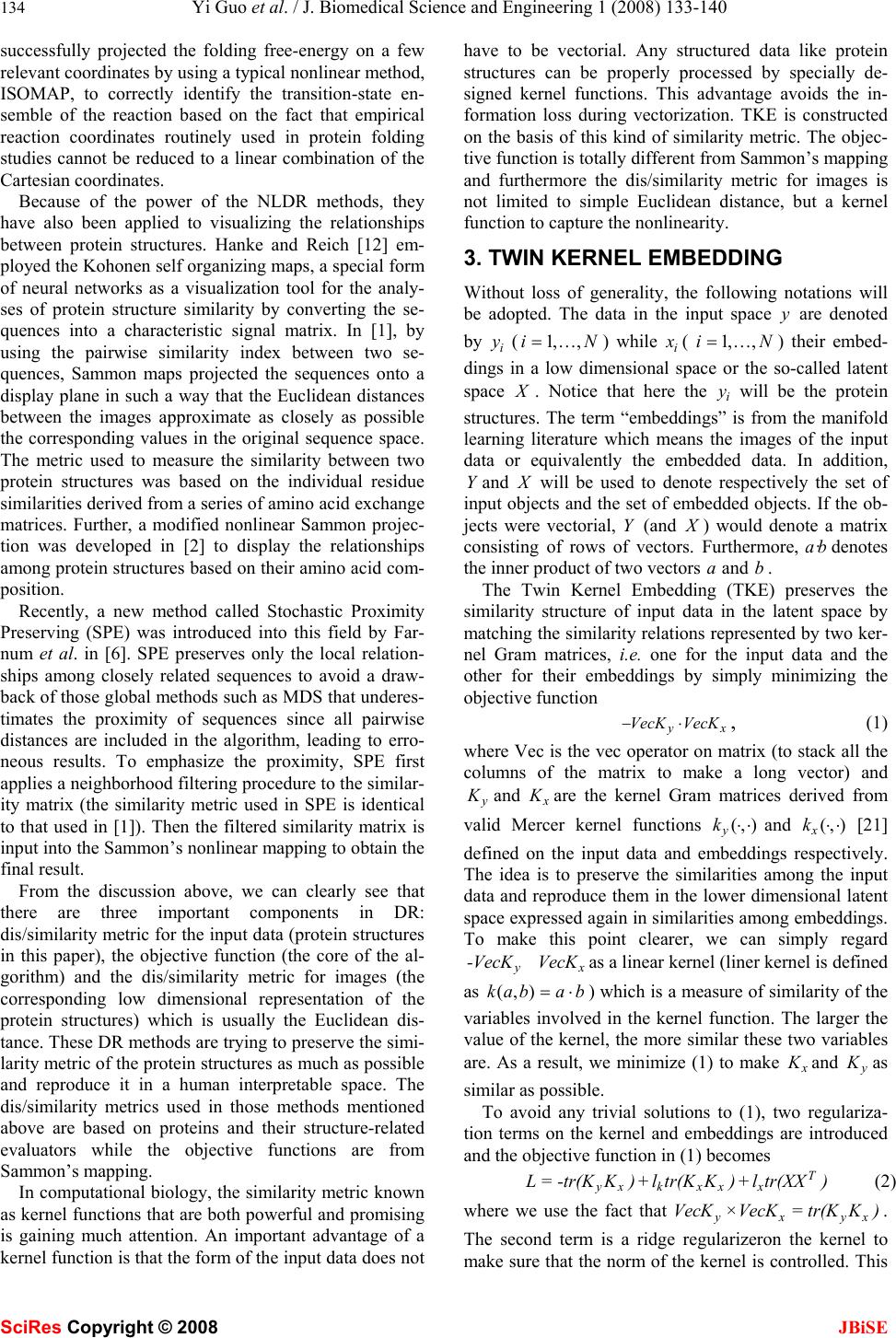

134 Yi Guo et al. / J. Biomedical Science and Engineering 1 (2008) 133-140
SciRes Copyright © 2008 JBiSE
successfully projected the folding free-energy on a few
relevant coordinates by using a typical nonlinear method,
ISOMAP, to correctly identify the transition-state en-
semble of the reaction based on the fact that empirical
reaction coordinates routinely used in protein folding
studies cannot be reduced to a linear combination of the
Cartesian coordinates.
Because of the power of the NLDR methods, they
have also been applied to visualizing the relationships
between protein structures. Hanke and Reich [12] em-
ployed the Kohonen self organizing maps, a special form
of neural networks as a visualization tool for the analy-
ses of protein structure similarity by converting the se-
quences into a characteristic signal matrix. In [1], by
using the pairwise similarity index between two se-
quences, Sammon maps projected the sequences onto a
display plane in such a way that the Euclidean distances
between the images approximate as closely as possible
the corresponding values in the original sequence space.
The metric used to measure the similarity between two
protein structures was based on the individual residue
similarities derived from a series of amino acid exchan ge
matrices. Further, a modified nonlinear Sammon projec-
tion was developed in [2] to display the relationships
among protein structures based on their amino acid com-
position.
Recently, a new method called Stochastic Proximity
Preserving (SPE) was introduced into this field by Far-
num et al. in [6]. SPE preserves only the local relation-
ships among closely related sequences to avoid a draw-
back of those global methods such as MDS that underes-
timates the proximity of sequences since all pairwise
distances are included in the algorithm, leading to erro-
neous results. To emphasize the proximity, SPE first
applies a neighborhood filtering procedure to the similar-
ity matrix (the similarity metric used in SPE is identical
to that used in [1]). Then the filtered similarity matrix is
input into the Sammon’s nonlinear mapping to obtain the
final result.
From the discussion above, we can clearly see that
there are three important components in DR:
dis/similarity metric for the input data (protein structures
in this paper), the objective function (the core of the al-
gorithm) and the dis/similarity metric for images (the
corresponding low dimensional representation of the
protein structures) which is usually the Euclidean dis-
tance. These DR methods are trying to preserve the simi-
larity metric of the protein structures as much as possible
and reproduce it in a human interpretable space. The
dis/similarity metrics used in those methods mentioned
above are based on proteins and their structure-related
evaluators while the objective functions are from
Sammon’s mapping.
In computational biology, the similarity metric known
as kernel functions that are both powerful and promising
is gaining much attention. An important advantage of a
kernel function is that the form of the input data does not
have to be vectorial. Any structured data like protein
structures can be properly processed by specially de-
signed kernel functions. This advantage avoids the in-
formation loss during vectorization. TKE is constructed
on the basis of this kind of similarity metric. The objec-
tive function is totally different from Sammon’s mapping
and furthermore the dis/similarity metric for images is
not limited to simple Euclidean distance, but a kernel
function to capture the nonlinearity.
3. TWIN KERNEL EMBEDDING
Without loss of generality, the following notations will
be adopted. The data in the input space y are denoted
by i y (,,1iN
=
…
) while i
x
( ,,1iN=… ) their embed-
dings in a low dimensional space or the so-called latent
space
X
. Notice that here the i y will be the protein
structures. The term “embeddings” is from the manifold
learning literature which means the images of the input
data or equivalently the embedded data. In addition,
Yand
X
will be used to denote respectively the set of
input objects and the set of embedded objects. If the ob-
jects were vectorial, Y (and
X
) would denote a matrix
consisting of rows of vectors. Furthermore, ·abdenotes
the inner product of two vectors aand b.
The Twin Kernel Embedding (TKE) preserves the
similarity structure of input data in the latent space by
matching the similarity relations represented by two ker-
nel Gram matrices, i.e. one for the input data and the
other for their embeddings by simply minimizing the
objective function
xy VecKVecK ⋅
−
, (1)
where Vec is the vec operator on matrix (to stack all the
columns of the matrix to make a long vector) and
y
K
and
x
K
are the kernel Gram matrices derived from
valid Mercer kernel functions (,)
y
k⋅⋅ and (,)
x
k
⋅
⋅ [21]
defined on the input data and embeddings respectively.
The idea is to preserve the similarities among the input
data and reproduce them in the lower dimensional latent
space expressed again in similarities among embeddings.
To make this point clearer, we can simply regard
yx
-ecK VecVKas a linear kernel (liner kernel is defined
as (,)kabab
=
⋅) which is a measure of similarity of the
variables involved in the kernel function. The larger the
value of the kernel, the more similar these two variables
are. As a result, we minimize (1) to make
x
K
and y
K
as
similar as possible.
To avoid any trivial solutions to (1), two regulariza-
tion terms on the kernel and embeddings are introduced
and the objective function in (1) becomes
yT xkxxx
L =-tr(KK)+ltr(KK)+ltr(XX) (2)
where we use the fact that yxyx ×Vec =tr(VecKKKK).
The second term is a ridge regularizeron the kernel to
make sure that the norm of the kernel is controlled. This

Yi Guo et al. / J. Biomedical Science and Engineering 1 (2008) 133-140 135
SciRes Copyright © 2008 JBiSE
can avoid solutions that simply let the elements in
x
K
go
to infinity. The third term imposes a heavy penalty on
too large a norm for the embeddings which ensure that
their coordinates are relatively small. k
λ
and
x
λ
are tun-
able parameters to control the strength of the regulariza-
tion and are assumed to be positive.
In order to capture the nonlinear structure,
(,)
x
k⋅⋅ should be chosen to be nonlinear. Normally, we
use the RBF kernel 2
ij
xi jx-x
k(x ,x)= gexp(-s)
2
‖‖
(3)
where
γ
and
σ
are positive hyperparameters. Nonethe-
less, other kernels can also be applied here. The selection
of RBF kernel is for its connection to the Euclidean dis-
tance which has a geometric understanding of the em-
beddings. There is no closed form solution for Xand
hence an optimization procedure like gradient descent
based algorithm for optimization should be employed
provided that (,)
x
k⋅⋅is differentiable. The initialization
of Xis also required to start the optimization process.
KLE [9], KPCA [22] and other methods that can work
with kernels could be utilized here for initializing
X
.
The dimension of the embeddings which is normally 2 is
assigned according to the application. A by-product of
this optimization process is that we can get the optimal
hyper-parameters (such as
γ
and
σ
if RBF kernel is used)
of the kernel function (,)
x
k⋅⋅as well. It ensures that the
kernel we pick up is well adjusted.
TKE is designed to preserve locality and non-locality
at the same time. This is done by the filtering of the en-
tries in y
K
. Not all the entries remain the same in the
optimization process but those that convey most of the
similarity information of the input data. This filtering
process is fulfilled by performing k-nearest neighbor
selecting procedure on y
K
. Given an object i y in the
input space, only those objects whose similarities (in the
sense of kernel values) to i
y are in the k nearest
neighbors that are selected to retain their original values
while all others are set to 0. The variable k (>1) in k-
nearest neighboring controls the neighborhood that the
algorithm will preserve. It can be interpreted as con-
structing a weighted adjacency graph which performs in
feature space and the weights on edges are evaluated by
a kernel as that in KLE. Similar procedure is involved in
SPE as well which uses the neighborhood radius to en-
sure the proximity preserving property. Because TKE
tries to match
x
K
to y
K
and RBF kernel (3) cannot give
a value of 0 except that two points in the latent space are
very far apart, TKE seeks a solution that keeps the points
in the same neighborhood close while makes the points
not in the same neighborhood be very far. However,
TKE also works without filtering in which case TKE
will preserve all pairwise similarities and will become a
global approach simply.
In addition to the fact that TKE outperforms other
methods such as KPCA, KLE etc, an elegant feature of
TKE is that it uses only the pairwise similarities since in
its objective function, only the kernel Gram matrix of the
input data is required. Through TKE, any kind of data
can be visualized in lower dimensional space as long as
an appropriate kernel is defined for them. As a result, a
kernel Gram matrix on the input data y K and an initiali-
zation for X will be adequate for TKE to find the opti-
mal embeddings.
4. CONSTRAINED TWIN KERNEL EM-
BEDDING
It is clear from observing (2) that there is no explicit
connections between input data and their corresponding
embeddings in TKE except the similarity preserving. As
such, the information hidden in the input data is ne-
glected. For example, if the input data actually stay on or
near to a smooth manifold embedded in the ambient
space, the location of the input data can be explored to
predict the coordinates of the embeddings on the mani-
fold. Furthermore, TKE can only find the optimal em-
beddings for currently presented data as we can see from
its objective function. To address these problems, we
introduce the constraints reflecting the relationship be-
tween input data and embeddings into TKE by following
steps. We first define a mapping function :
f
yx→and
then incorporate it into the objective functional of TKE
as regularization terms. Finally the optimal embeddings
X and the
f
will be searched via conjugate gradients
algorithm.
We can start from the kernel feature mapping directly
and incorporate it as the core part of the LS-SVM (the
dual form of the objective function of LS-SVM) into
TKE as what has been done in [24]. We minimize the
following objective function similar to that of LS-SVM
with equality constraints
d2
j
jij
j=1 i
T
j
uh
J
=ww+e
22
∑
∑ (4)
. ()
T
ijj jiij
s
.t xye ωϕ
=
+ (5)
corresponding to the maximum margin (the first term)
and least square errors (the second term) in (4) where
υ
and
η
are adjustable parameters.
j
ϕ
’s are the feature
mappings which map the input i y into Hilbert space
where the inner product is defined.
j
ω
is a column vec-
tor having the same dimension as the Hilbert space. We
can regard the i
x
in (5) as the projection of ()
i
y
ϕ
onto
a subspace parameterized by
j
ω
’s. Because the differ-
ence of the constraints, it does not have the same geo-
metrical interpretation of LS-SVM because the original
constraints are inequalities reflecting the correct classifi-
cation hyperplanes while here they are just feature map-

136 Yi Guo et al. / J. Biomedical Science and Engineering 1 (2008) 133-140
SciRes Copyright © 2008 JBiSE
ping which builds the relation between input data i y and
its counterpart i
x
in low dimensional space. In (4), we
are minimizing the error ij e in reconstruction of i
x
es-
sentially however it should be done with ij
ω
properly
constrained. This happens to have the form of the LS-
SVM objective function. To solve (4) with the equality
constraints (5), we can use Lagrange multipliers as
dT2
j
jijijijjjiij
j=1ij ij
T
uh
L
=ww+e+a(x-wf(y)-e)
22
∑∑∑ (6)
From the saddle points, 0
j
L
ω
∂
∂
=
, 0
ij
L
e
∂=
∂ we have
1
() 0()
.
1
0
j
ijj ijijj i
jii
ij ijijij
ij
L
Lee
e
υωα ϕωα ϕ
ωυ
ηα α
η
∂=− =⇒=
∂
∂=−=⇒=
∂
∑∑
yy
Substitute them back into (6) and eliminate
j
ω
and ij
e
we have the dual problem to be maximized according to
the min-max duality
d2
ijji ijjiij
j=1 iiij
ijijijjij iij
ij i
2
jjjijij
jijij
T
T
i
T
j
u11 h1
L=(af (y )) (af(y ))+(a)
2u u 2h
11
+a {x-(af (y ))f(y )-a}
uh
11
=-aK a-a+a x
2u 2h
∑∑∑ ∑
∑∑
∑∑∑
(7)
where 1T
2
(,, )
jj j
αα α =… , ()()()
mij
Tmi
yyky,y ϕϕ =
to which the “kernel trick” applies. (,)
j
k⋅⋅ is the kernel
associated with the kernel mapping and
j
K
is the Gram
matrix derived from (,)
j
k⋅⋅ accordingly. We then maxi-
mize the above dual problem with respect to ij
α
instead
of
j
ω
and ij e. From the discussion above we see that
the ij
x
’s are free variables. To limit the choice of them,
we combine (7) with the objective functional of TKE to
incorporate the similarity preserving as
2
yij xi jkxi jxii
i,jij i
2
jjij ij
T
Tij
jiji
jj
L=-k (y,y)k(x,x)+lk (x,x)+lxx
11
+aKa+a-ax
2u 2h
∑∑∑
∑∑∑ (8)
where we turn the maximization of (7) to minimization
aligned with the TKE objective functional. Here we see
that the terms related to i y are expressed by kernel
(,)
y
k⋅⋅ . Therefore, this revised objective function is still
non-vectorial data applicable. Again we express (8) into
matrix form to facilitate the differentiation and let
(,) (,)
yj
kk⋅⋅ =⋅⋅ for simplicity
T
TT
2
xy k xx
yT
L=-tr[KK+ lK+ lXX
11
+tr[AKA]+tr[A A]-tr[A X]
2u 2
]tr[]t[
h
r]
(9)
where
11 1d
N1 Nd
a
A= MM
a
⎡
⎤
⎢
⎥
⎢
⎥
⎢
⎥
⎣
⎦
Hence we minimize L in (8) with respect to
A
,
X
and
kernel hyperparameters of (,)
x
k⋅⋅. If we substitute the
saddle point solution back into the equality constraints
(5), the following mapping function is handy to predict
new input samples
ijmj ymiij
m
11
x
=ak(y,y)+a
uh
∑ (10)
The errors 1ij
α
η
can be neglected since the values of the
errors are very small compared with
X
after optimiza-
tion.
To apply the conjugate gradient algorithm, the deriva-
tives of L with respect to X and Aare given by
,and, 2
xkx y
xx
LLK L
A
K-K
XKX K
λ
∂∂∂ ∂
=− =
∂∂∂ ∂ (11)
11
y
L
K
AA-X
A υη
∂=+
∂ (12)
X
is still initialized by KPCA or KLE to obtain pure
non-vectorial data applicability. Initial
A
is from the
solution of 0
L
A
∂
=
∂ after
X
is known. We have
11
(-1
y
A
KI)X
υη
=+ . It implies that we could alternately
update
X
and
A
in optimization, however we still use
conjugate gradient algorithm to update them at the same
time. Because the mapping function defined between
input space and latent space acts as constraints, we call
this algorithm Constrained TKE (CTKE). It is noticeable
that in CTKE, we use y
K
to construct the mapping
function, so we do not have to filter y
K
before com-
mencing the algorithm.
5. EXPERIMENTAL RESULTS
Experiments were conducted on the SCOP (Structural
Classification Of Protein). This database is available at
http://scop.mrc-lmb.cam.ac.uk/scop/. The database
comes with a detailed and comprehensive description of
the structural and evolutionary relationships of the pro-
teins of known structure. 292 protein structures from
different protein superfamilies and families are extracted
for the test. The kernels we used are from the family of
the so-called alignment kernels whose thorough analyses
can be found in [18]. The corresponding kernel Gram
matrices are available on the website of the paper as
supplements and were used directly in our experiments.
5.1 Parameters Setting
Both CTKE and TKE have parameters to be determined
beforehand. Through empirical analyses (performed a set

Yi Guo et al. / J. Biomedical Science and Engineering 1 (2008) 133-140 137
SciRes Copyright © 2008 JBiSE
of experiments on the same data set varying only the
parameters), we found these algorithms are not sensitive
to the choice of the parameters, so long as the conjugate
gradient optimization can be carried out without prema-
ture early stop. So we use the following parameters in
the 10k= in k nearest neighboring; for CTKE,
0.05
k
λ
=, experiments. For TKE, 0.005
k
λ
=
,
0.001
x
λ
=
and 0.01
x
λ
=
,0.5
υ
η == . The minimize
tion will stop after 1000 iterations or when consecutive
update of the objective function is less than 7 10-.(,)
x
k
⋅
⋅
is the RBF kernel and initialization is done by KPCA for
both CTKE and TKE.
(a) CTKE with MAMMOTH kernel
(b) TKE with MAMMOTH kernel
Figure 1. Visualization results of protein structures.

138 Yi Guo et al. / J. Biomedical Science and Engineering 1 (2008) 133-140
SciRes Copyright © 2008 JBiSE
5.2 Proteins on 2-D Plane
The proteins from the same families are expected to be
close in the 2-dimensional space with overlappings indi-
cating similar proteins but actually from different fami-
lies. The results are plotted in Figure 1. The results of
other methods (kernel applicable methods) are also pre
sented for comparison in Figure 2. Each point (denoted
as a shape in the figures) represents a protein. The same
shapes with the same colors are the proteins from same
families while the same shapes with different colors rep-
resent the proteins from different families but of thesame
superfamilies. All the figures in this paper share the
same legends as those in Figure 1 (b).
Both TKE and CTKE reveal the fact that proteins
from the same families congregate together as clusters
while KPCA and KLE fail to reveal it. For example, in
Figure 1 (a) and (b), almost all of the proteins from the
globin family gathered at the bottom left corner indicat-
ing similar structures. Interestingly, CTKE and TKE also
reveals the fact that the proteins from the same super-
family but different families are similar in structure,
which is reflected in the 2-dimensional plane that the
corresponding groups (families) are close if they are in
the same superfamily. For instance, note that the proteins
from ferritin and ribonucleotide reductase-like families
(blue diamonds and violet diamond respectively in the
figure), they are close in the group level. SPE has com-
parable performance visually. But the overlapping in the
middle shows that it cannot distinguish some families
clearly.
In order to further quantify the results, we use the “pu-
rity” [8] to evaluate some of these methods. It uses the
fraction of the number of samples from the same class as
given point in a neighborhood with size n. The purity is
the average of the fraction over all points. The higher the
purity, the better the quality of the clusters. Intuitively,
this standard provides an objective judgement from the
classification point of view and the method with better
(a) KPCA (b) KLE (k = 50)
(c) SPE (global) (d) SPE (local k = 100)
Figure 2. The result of other methods with MAMMOTH kernel. Like TKE, SPE can work globally and locally depending on
whether the kernel Gram matrix is filtered first by k-nearest neighboring. SPE global worked with the whole kernel Gram matrix
and SPE local filtered Ky with 100-nearest neighboring in this experiment

Yi Guo et al. / J. Biomedical Science and Engineering 1 (2008) 133-140 139
SciRes Copyright © 2008 JBiSE
Figure 3. Comparison of different methods using purity.
purity has the potential to achieve better classification
rate. It is noticeable that for SPE and KLE with parame-
ter k, we did multiple experiments to choose the optimal
value of k corresponding to the largest purity when the
size of neighborhood is 1. We found that for SPE the
larger the k, the better the result. Specifically, when k
equals the number of the data, i.e. n o filtering at all, SPE
turns out to be a nonlinear MDS. As we can see from
Figure 3, CTKE and TKE have higher purity than others.
The average purity of CTKE is 0.5946 and TKE 0.6135.
It shows that CTKE has very close performance to TKE.
However, the advantage of the CTKE is its ability to
predict novel samples because of the mapping function
defined explicitly between input space and latent space.
This mechanism broadens the applicability of this algo-
rithm greatly to classification, identification etc. It also
provides a tool to explore the manifold formed by data.
6 CONCLUSIONS
In this paper, we visualized the similarity relationships
among protein structures using constrained Twin Kernel
Embedding (CTKE) which is constructed on the original
TKE [10]. It has comparable performance to that of TKE
but possesses the ability to predict the embeddings for
novel samples. Because CTKE implements a mapping
function from input space to latent space, the information
among input data is further exploited. CTKE also has the
similarity preserving property as TKE does and is purely
non-vectorial data applicable since the mapping function
comes from the feature mapping and expressed as kernel
function eventually. Moreover, there is no k-nearest
neighbor filtering in CTKE and hence avoid choosing
another parameter which is common across other DR
algorithms. From the experiments on proteins, we have
seen that CTKE preserves the similarity relationships
among the protein structures and reproduces them in a
much lower dimensional space, allowing easy interpreta-
tion by researchers. This algorithm is promising as it can
be further applied to the study of the evolution of protein
structure and the prediction of proteins functions.
ACKNOWLEDGEMENTS
This work is supported by the National Science Foundation of China
(NSFC 60373090), the ARC DP Development Grant from Charles Sturt
University and the University Research Grant from the University of
New England.
REFERENCES
[1] Dimitris K. Agrafiotis. (1997) A new method for analyzing protein
sequence relationships based on sammon maps. Protein Science,
6(2):287–293.
[2] Izydor Apostol and Wojciech Szpankowski. (1999) Indexing and
mapping of proteins using a modified nonlinear sammon projection.
Journal of Computational Chemistry, 20 (10):1049– 1059.
[3] Mikhail Belkin and Partha Niyogi. (2003) Laplacian eigenmaps for
dimensionality reduction and data representation. Neural Computa-
tion, 15(6):1373–1396.
[4] Samarasena Buchala, Neil Davey, Ray J. Frank, and Tim M. Gale.
(2004) Dimensionality reduction of face images for gender classifi-
cation. In Proceedings of 2nd International IEEE Conference on In-
telligent Systems, volume 1, pages 88–93.
[5] Payel Das, Mark Moll, Hern´an Stamati, Lydia E. Kavraki, and
Cecilia Clementi. (2006) L owd imensional free energy landscapes of
protein folding reactions by nonlinear dimensionality reduction. In
Proceedings of the National Academy of Sciences, volume 103,
pages 9885– 9890, USA .
[6] Michael A. Farnum, Huafeng Xu, and Dimitris K. Agrafiotis. (2003)
Exploring the nonlinear geometry of protein homology. Protein
Science, 12(1604-1612) .
[7] Ronald A. Fisher. (1936) The use of multiple measurements in
taxonomic problems. Annals of Eugenics, 7:179–188 .
[8] Amir Globerson, Gal Chechik, Fernando Pereira, and Naftali
Tishby.(2005) Euclidean embedding of co-occurrence data. In Law-

140 Yi Guo et al. / J. Biomedical Science and Engineering 1 (2008) 133-140
SciRes Copyright © 2008 JBiSE
rence K. Saul, YairWeiss, and L´eon Bottou, editors, Advances in
Neural Information Processing Systems 17, pages 497–504. MIT
Press, Cambridge, MA .
[9] Yi Guo, Junbin Gao, and Paul W. Kwan. (2006) Kernel Laplacian
eigenmaps for visualization of non-vectorial data. In Lecture Notes
on Artificial Intelligence, volume 4304, pages 1179– 1183.
[10] Yi Guo, Junbin Gao, and Paul W. Kwan. (2008) Twin kernel em-
bedding. IEEE Transaction ofPattern Analysis and Machine Intel-
ligence, submitted.
[11] Jihun Ham, Yuanqing Lin, and Daniel. D. Lee. (2005) Learning
nonlinear appearance manifolds for robot localization. In
IEEE/RSJ International Conference on Intelligent Robots and Sys-
tems, pages 2971– 2976.
[12] Jens Hanke and Jens G. Reich. (1996) Kohonen map as a visuali-
zation tool for the analysis of protein sequences: multiple align-
ments, domains and segments of secondary structures. Bioinfor-
matics, 12(6):447–454.
[13] M. Jolliffe. (1986) Principal Component Analysis. Springer-
Verlag, New York.
[14] Philip M. Kim and Bruce Tidor. (2003) Subsystem identification
through dimensionality reduction of large-scale gene expression
data. Genome Research, 13:1706–1718.
[15] Nathan Mekuz, Christian Bauckhage, and John K. Tsotsos. (2005)
Face recognition with weighted locally linear embedding. In Pro-
ceedings of the 2nd Canadian Conference on Computer and Robot
Vision, pages 290–296.
[16] Oleg Okun, Helen Priisalu, and Alexessander Alves. (2005) Fast
non-negative dimensionality reduction for protein fold recognition.
In ECML, pages 665–672.
[17] Zhengjun Pan, Rod Adams, and Hamid Bolouri. (2000) Dimen-
sionality reduction of face images using discrete cosine transforms
for recognition. In IEEE Conference on Computer Vision and Pat-
tern Recognition. [18] Jian Qiu, Martial Hue, Asa Ben-Hur, Jean-
Philippe Vert, and William Stafford Noble. (2007) An alignment
kernel for protein structur es. In Bioinformatics.
[18] Bisser Raytchev, Ikushi Yoda, and Katsuhiko Sakaue. (2006)
Multi-view face recognition by nonlinear dimensionality reduction
and generalized linear models. In FGR ’06: Proceedings of the 7th
International Conference on Automatic Face and Gesture Recog-
nition (FGR06), pages 625–630, Washington, DC, USA.
[19] Sam T. Roweis and Lawrence K. Saul. (2000) Nonlinear dimen-
sionality reduction by locally linear embedding. Science,
290(22):2323–2326.
[20] B. Sch¨olkopf and A.J. Smola. (2002) Learning with Kernels:
Support Vector Machines, Regularization, Optimization, and Be-
yond. The MIT Press, Cambridge, MA.
[21] Bernhard Sch¨olkopf, Alexander J. Smola, and Klaus-Robert
M¨uller. (1998) Nonlinear component analysis as a kernel eigen-
value problem. Neural Computation, 10:1299–1319.
[22] J.A.K. Suykens and J. Vandewalle. (1999) Least squares support
vector machine class ifiers. Neural Processing Letters, 9:293–300.
[23] Johan A.K. Suykens. (2007) Data visualization and dimensionality
reduction using kernel maps with a reference point. Technical Re-
port 07-22, K.U. Leuven, ESAT-SCD/SISTA.
[24] Joshua B. Tenenbaum, Vin de Silva, and John C. Langford. (2000)
A global geometric framework for nonlinear dimensionality reduc-
tion. Science, 290(22):2319–2323.
[25] Miguel L. Teodoro, George N. Phillips Jr, and Lydia E. Kavraki.
(2002) A dimensionality reduction approach to modeling protein
flexibility. In International Conference on Computational Molecu-
lar Biology (RECOMB), pages 299–308.
[26] Miguel L. Teodoro, George N. Phillips Jr, and Lydia E. Kavraki.
(2003) Understanding protein flexibility through dimensionality
reduction. Journal of Computational Biology, 10(3-4):617–634