Journal of Geographic Information System, 2011, 3, 232-241
doi:10.4236/jgis.2011.33020 Published Online July 2011 (http://www.SciRP.org/journal/jgis)
Mapping Glacier Variations at Regional Sca le through
Equilibrium Line Altitude Interpolation: GIS and
Statistical Application in Massif des Écrins (French Alps)
Étienne Cossart
UMR Prodig 8586 – CNRS, Université Paris 1 – Panthéon Sorbonne, Paris, France
Received February 26, 201 1; revised April 13, 2011; accepted April 26, 2011
Abstract
Glacier variation is one of the best indicators of climate change in mountainous environment. In French Alps,
many temporal data are acquired by glaciologists at glaciers scale: geometrical parameters (surface area,
thickness, length and front altitude) are surveyed since the end of the 19th century. Those parameters are
necessary to estimate the mass-balance of glaciers and, then, an accurate temporal signal of glacier variation.
However, the time-response of the glaciers can be highly variable because of the topoclimate, and more gen-
erally the local settings of the glaciers. Moreover, climatologists and hydrologists are requiring estimation of
glacier variations at regional scale and not only at local scale. In this paper, we highlight that the Equilibrium
Line Altitude (ELA) is a parameter prone to spatio-temporal reconstructions at regional scale. ELA can in-
deed be interpolated at a region scale from local data: for instance, many geographers have reconstructed
spatial trends during 1980s. Here, we try to interpolate ELA from multi-dimensionnal regression analysis:
ELA is explained by many local parameters (Incoming solar radiation, topographic indexes, snow-redistribu-
tion by wind, etc.). Regression model was adjusted from a spatio-temporal database of 50 glaciers, located in
the Massif des Écrins. ELA was estimated for each glacier thanks to the Accumulation Area Ratio (ratio =
0.65) at two stages: LIA maximum and at present. Results first show that the multiple regression analysis is
efficient to interpolate ELA through space: the adjusted r² is about 0.49 for the reconstruction during the LIA,
and 0.47 at present. Moreover, the RMSE error is about 50 meters for the LIA period, 55 meters at present.
Finally, a high spatial variability (standard deviation of about 150 meters) is highlighted: incoming solar ra-
diation and snow redistribution by wind mostly explain the observed differences. We can also assess a rise of
the ELA of about 250 meters during the 20th century.
Keywords: Glaciers, Equilibrium line, Interpolation, GIS, Massif des Écrins, Alps
1. Introduction
The current debate on the climate change has highlighted
the importance of glaciers, as their evolution may be a
good proxy of temperatures and precipitations variation.
Moreover, glacier melting may induce significant modi-
fication on river regime and, more generally, on water
resource availability. Glacier survey has hitherto mostly
involved glaciologists, that provided precise topographic
measurements (surface area, length, thickness variation,
etc.) to compute mass-balance. Those data were acquired
on very few glaciers, that were carefully investigated
through time (once or many times a year); in the Alps,
those series often began at the end of the 19th century
[1-5]. The main problem of such database is that sur-
veyed glaciers are isolated in space, hampering any con-
sideration at a regional scale. Geographers can indeed
ask if surveyed glacier may reveal a regional scenario or
if their evolution patterns only reflect local settings. For
instance asynchronicity between glaciers was empha-
sized at various scales: from a continental scale [6] to
local scale [7]. Firstly, within a mountainous region, it
has been observed that glacier variation may be due to
exposure to humid fluxes: in the Alps, well-exposed gla-
ciers (eastern glaciers) are asynchronous with glaciers
that are sheltered from humid fluxes (western glaciers)
[8,9]. Secondly, it is known since the beginning of the
20th century that glaciers may be characterized by dif-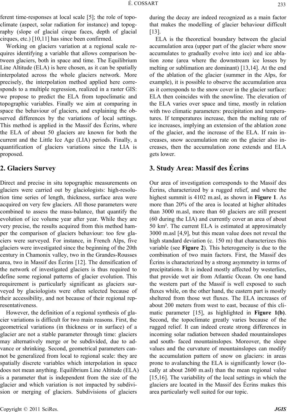

É. COSSART
233
ferent time-responses at local scale [5]; the role of topo-
climate (aspect, solar radiation for instance) and topog-
raphy (slope of glacial cirque faces, depth of glacial
cirques, etc.) [10,11] has since been confirmed.
Working on glaciers variation at a regional scale re-
quires identifying a variable that allows comparison be-
tween glaciers, both in space and time. The Equilibrium
Line Altitude (ELA) is here chosen, as it can be spatially
interpolated across the whole glaciers network. More
precisely, the interpolation method applied here corre-
sponds to a multiple regression, realized in a raster GIS:
we propose to predict the ELA from topoclimatic and
topographic variables. Finally we aim at comparing in
space the behaviour of glaciers, and explaining the ob-
served differences by the variations of local settings.
This method is applied in the Massif des Écrins, where
the ELA of about 50 glaciers are known for both the
current and the Little Ice Age (LIA) periods. Finally, a
quantification of glaciers variations since the LIA is
proposed.
2. Glaciers Survey
Direct and precise in situ topographic measurements on
glaciers were carried out by glaciologists: high-resolu-
tion time series of length, thickness, surface area were
acquired on very few glaciers. All those parameters were
combined to assess the mass-balance, that quantify the
evolution of ice volume year after year. While they are
very precise, the results acquired from this method ham-
per the comparison of glaciers behaviour: too few gla-
ciers were surveyed. For instance, in French Alps, five
glaciers were investigated since the beginning of the 20th
century in Chamonix valley, two in the Grandes-Rousses
area, two in Massif des Écrins [12]. The densification of
the network of investigated glaciers is thus required to
define some regional patterns of glacier evolution. This
requirement is particularly significant as glaciers sur-
veyed by glaciologists were often selected because of
their accessibility, and not because of their regional rep-
resentativeness.
However, the definition of a regional synthesis of gla-
cier variations is difficult for two main reasons. First, the
geometrical variations (in thickness or in surface) of a
glacier are not a stable parameter through time: glaciers
may alternatively merge or be subdivided, due to ad-
vance or shrinking. Second, geometrical parameters can-
not be generalized from local to regional scale: they are
spatially discrete variables which interpolation in space
does not mean anything. Equilibrium Line Altitude (ELA)
is a parameter that is independent from the size of the
glacier and which variation is not impacted by subdivi-
sion or merging of glaciers. Subdivisions of glaciers
during the decay are indeed recognized as a main factor
that makes the modelling of glacier behaviour difficult
[13].
ELA is the theoretical boundary between the glacial
accumulation area (upper part of the glacier where snow
accumulates to gradually evolve into ice) and ice abla-
tion zone (area where the downstream ice losses by
melting or sublimation are dominant) [13,14]. At the end
of the ablation of the glacier (summer in the Alps, for
example), it is possible to observe the accumulation area
as it corresponds to the snow cover in the glacier surface:
ELA then coincides with the snowline. The elevation of
the ELA varies over space and time, mostly in relation
with two climatic parameters: precipitation and tempera-
tures. If temperatures increase, then the melting rate of
ice increases, implying an extension of the ablation zone
of the glacier, and the increase of the ELA. If rain in-
creases, snow accumulation rate on the glacier also in-
creases, then the accumulation zone extends and ELA
gets lower.
3. Study Area: Massif des Écrin s
Our area of investigation corresponds to the Massif des
Écrins, characterized by a rugged relief, and where the
highest summit is 4102 m.asl, as shown in Figure 1. As
more than 20% of the area is located at higher altitudes
than 3000 m.asl, more than 60 glaciers are still present
(60 during the LIA) and currently cover an area of about
50 km². The current ELA is estimated at approximately
3000 m.asl [4,9], but this mean value does not reveal the
high standard deviation (c. 150 m) that characterizes this
variable (see Figure 2). This heterogeneity is due to the
combination of two main factors. First, the Massif des
Écrins is characterized by a strong asymmetry in terms of
precipitations. It is indeed mostly affected by westerlies,
that provide wet air from Atlantic Ocean. On one hand
the western part of the Massif is well exposed to such
fluxes while, on the other hand , the eastern part is mostly
sheltered from those wet fluxes. The ELA increases of
about 200 meters from west to east, because of this cli-
matic parameter [15], as highlighted in Figure 1(b).
Second, the topoclimate greatly varies because of the
rugged relief. It can indeed create strong differences in
incoming solar radiation between shaded mountainslopes
and south- faced mountainslopes. Moreover, the slope
values and the curvature of mountainslopes can modify
the accumulation pattern of snow on glaciers: in areas
prone to avalanching the ELA is significantly lower (lo-
cally at about 2600 m.asl) than the mean regional value
[15,16]. The variability of the local setting s in which the
glaciers are located in the Massif des Écrins makes this
area particularly well suited for our topic.

É. COSSART
234
Figure 1. Study area. A: location map; B: Climatic gradient from west to east; C: Topography of the study area.
Figure 2. ELA database during the LIA and at prese nt. Left: Statistical distribution of ELA; Right: Variogram.

É. COSSART
235
4. Methods
4.1. Database Acquisition
Several methods exist to estimate the altitude of the
equilibrium line [17,18], most of them are based upon a
geometric reconstruction of glacier extents. It is indeed
commonly considered that the surface area of the accu-
mulation zone corresponds to the upper two-thirds (in
terms of altitude) of the glacier area, the ablation zone
then corresponding to the lower third [14,19]. A map of
glacier extent, combined with a topographical template,
thus allows the reconstruction of the altitudinal distribu-
tion of ice area and then the estimation of the position of
the ELA. The ELA assessment, acquired for different
glaciers and at different dates, provides a basic spa-
tio-temporal database that corresponds to an inventory of
the glaciers located in the Massif des Écrins, at both LIA
and present stages.
Little Ice Age ELA are estimated from geographical
reconstruction of glacier extents—based upon geomor-
phic criteria [20,21] and archives [21,23]. The extents of
57 glaciers were reconstructed and integrated within a
GIS (SAGA GIS). Current ELA are estimated thanks to
aerial photographs (Institut Géographique National –IGN–)
and field investigation. More precisely, 63 glaciers were
observed through fieldwork and aerial photographs (ac-
quired in 2004), and mapped within the GIS. All glaci-
ated areas were combined with a DEM (provided by In-
stitut Géographique National) within SAGA GIS to fi-
nally assess the hypsometric curve of each glacier. From
this hypsometric curve, the ELA was estimated at both
stages and summarized in Figure 2.
During the LIA, the mean ELA was about 2750 m.asl
(2763 m.asl, standard deviation = 174 m), while at pre-
sent it is about 3000 m.asl (3024 m.asl, standard devia-
tion = 175 m). A high heterogeneity is emphasized
through the variograms in Figure 2; even if the glaciers
are close, as shown by the variogram calculated for both
periods. These characteristics hampered any application
of classical methods of interpolation based upon the dis-
tance, such as IDW or even kriging.
4.2. Predictor Variables
As suggested by the standard deviation at both dates,
local settings of each glacier play a major role to differ-
entiate the ELA in space. If we realize an inventory of all
variables that can locally influence the ELA, three clus-
ters of predictor variables can be highlighted. First, at a
regional scale, latitude and longitude can highly influ-
ence the ELA variation. In the present study, latitude
indeed reflects the distance to the Mediterranean Sea and
longitude the distance from Atlantic Ocean. Those two
variables thus take into account the distance from humid
sources, which role is of ten highlighted in previous stud-
ies [3,6,24]. Second, variables defining the topoclimate
should be considered. Of course, the incoming solar ra-
diation, which is varying significantly in mountainous
areas, is of prime importance. We also pay attention to
the wind, that can redistribute significant quantities of
snow: an identification of deflation/accumulation area
through the dominant winds (N260˚) was simulated
through SAGA GIS. Third, all topographical variables
that influence the accumulation of snow by avalanching
are assessed: slope, curvature, length of mountain slopes
[10]. They were all calculated from a DEM through
SAGA GIS software. The DEM we used was provided
by IGN, and is characterized by an altitude accuracy of 5
meters, while pixels are 20-meter large. To avoid any
boundary effect during the calculations, we decided to
assess the predictor variables on an area larger than the
study area: a buffer of five kilometers was each time
considered.
4.3. Method of interpolation
The first attempts of ELA interpolation were realized
during the 1970s by fitting an order one regression plane
in space [6,25]: the spatial variation of ELA was then
mostly explained by latitude and longitude, particularly
in order to highlight precipitations gradients. More re-
cently we tried to minimize the residual scores b y apply-
ing methods defined by climatologists. Interpolation was
then made in two steps: first by fitting a polynomial law
surface (order 2 or 3) expressing the ELA as a function
of latitude and longitude, second by kriging the residual
scores [26]. However, such methods are not useful to
explain what are the main predictors contributing to the
spatial variation of ELA. Another method is thus to real-
ize a multiple regression between ELA and the predictor
variables identified previously.
As all the predictor variables can be represented in
space by a grid, most of the procedure can be made
through SAGA GIS software. First, for each glacier, the
values of pr ed ictor variables are summarized. At this step
we consider not only the glacier itself, but also the
catchment located above the glacier, as it plays a major
role in snow accumulation. Correlation coefficients are
presented in Table 1. Then, a stepwise (descending)
multiple regression was made in R software for LIA and
Present data, with all the predictors variables. Thanks to
adjusted R², we only selected all the predictors that con-
tribute significantly to the variation of ELA, and then
computed another regression model. This procedure was
realized many times, until the value of the adjusted R²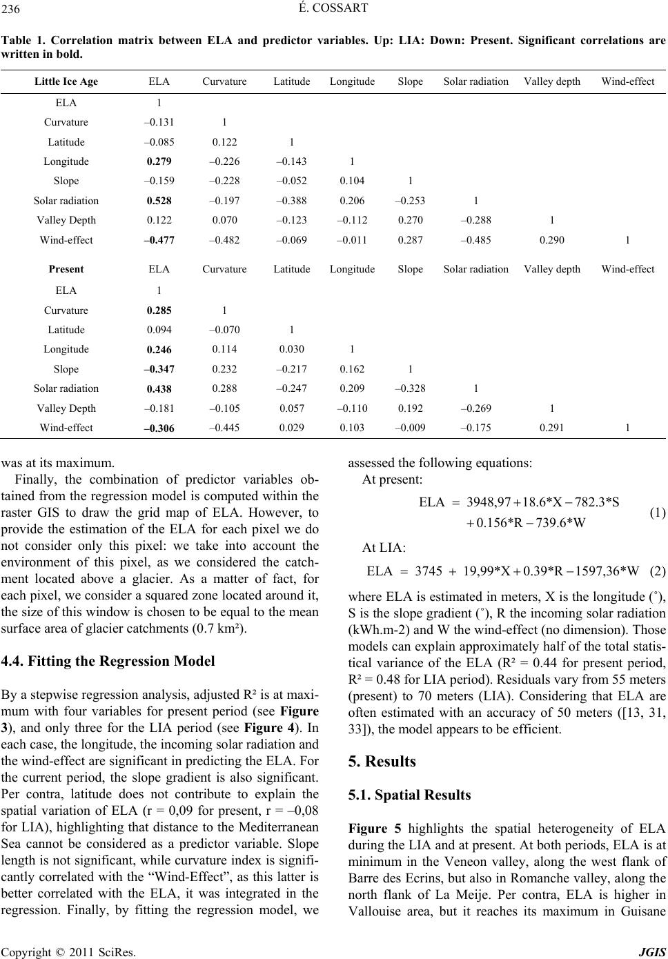

É. COSSART
236
Table 1. Correlation matrix between ELA and predictor variables. Up: LIA: Down: Present. Significant correlations are
written in bold.
Little Ice Age ELA Curvature Latitude LongitudeSlope Solar radiation Valley depth Wind-effect
ELA 1
Curvature –0.131 1
Latitude –0.085 0.122 1
Longitude 0.279 –0.226 –0.143 1
Slope –0.159 –0.228 –0.052 0.104 1
Solar radiation 0.528 –0.197 –0.388 0.206 –0.253 1
Valley Depth 0.122 0.070 –0.123 –0.112 0.270 –0.288 1
Wind-effect –0.477 –0.482 –0.069 –0.011 0.287 –0.485 0.290 1
Present ELA Curvature Latitude LongitudeSlope Solar radiation Valley depth Wind-effect
ELA 1
Curvature 0.285 1
Latitude 0.094 –0.070 1
Longitude 0.246 0.114 0.030 1
Slope –0.347 0.232 –0.217 0.162 1
Solar radiation 0.438 0.288 –0.247 0.209 –0.328 1
Valley Depth –0.181 –0.105 0.057 –0.110 0.192 –0.269 1
Wind-effect –0.306 –0.445 0.029 0.103 –0.009 –0.175 0.291 1
wa s at its maximum.
Finally, the combination of predictor variables ob-
tained from the regression model is computed within the
raster GIS to draw the grid map of ELA. However, to
provide the estimation of the ELA for each pixel we do
not consider only this pixel: we take into account the
environment of this pixel, as we considered the catch-
ment located above a glacier. As a matter of fact, for
each pixel, we consider a squared zone located around it,
the size of this window is chosen to be equal to the mean
surface area of glacier catchments (0.7 km²).
4.4. Fitting the Regression Model
By a stepwise regression analysis, adjusted R² is at maxi-
mum with four variables for present period (see Figure
3), and only three for the LIA period (see Figure 4). In
each case, the longitude, the incoming solar radiation and
the wind-effect are significant in predicting the ELA. For
the current period, the slope gradient is also significant.
Per contra, latitude does not contribute to explain the
spatial variation of ELA (r = 0,09 for present, r = –0,08
for LIA), highlighting that distance to the Mediterranean
Sea cannot be considered as a predictor variable. Slope
length is not significant, while curvature index is signifi-
cantly correlated with the “Wind-Effect”, as this latter is
better correlated with the ELA, it was integrated in the
regression. Finally, by fitting the regression model, we
assessed the following equations :
At present:
ELA 3948,9718.6*X782.3*S
0.156*R 739.6*W


 (1)
At LIA:
ELA 3745 19,99*X0.39*R1597,36*W

 (2)
where ELA is estimated in meters, X is the longitude (˚),
S is the slope gradient (˚), R the incoming solar radiation
(kWh.m-2) and W the wind-effect (no dimension). Those
models can explain approximately half of the total statis-
tical variance of the ELA (R² = 0.44 for present period,
R² = 0.48 for LIA period). Residuals vary from 55 meters
(present) to 70 meters (LIA). Considering that ELA are
often estimated with an accuracy of 50 meters ([13, 31,
33]), the model appears to be efficient.
5. Results
5.1. Spatial Results
Figure 5 highlights the spatial heterogeneity of ELA
during the LIA and at presen t. At both periods, ELA is at
minimum in the Veneon valley, along the west flank of
Barre des Ecrins, but also in Romanche valley, along the
north flank of La Meije. Per contra, ELA is higher in
Vallouise area, but it reaches its maximum in Guisane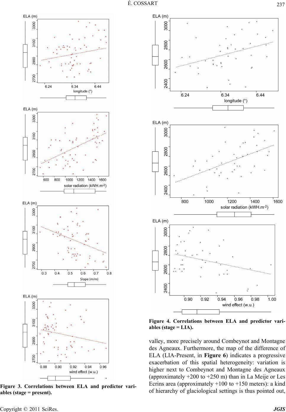

É. COSSART
237
Figure 3. Correlations between ELA and predictor vari-
ables (stage = present).
Figure 4. Correlations between ELA and predictor vari-
ables (stage = LIA).
valley, more precisely around Combeynot and Montagne
des Agneaux. Furthermore, the map of the difference of
ELA (LIA-Present, in Figure 6) indicates a progressive
exacerbation of this spatial heterogeneity: variation is
higher next to Combeynot and Montagne des Agneaux
(approximately +200 to +2 50 m) than in La Meije or Les
Ecrins area (approximately +100 to +150 meters): a kind
of hierarchy of glaciological settings is thus pointed out,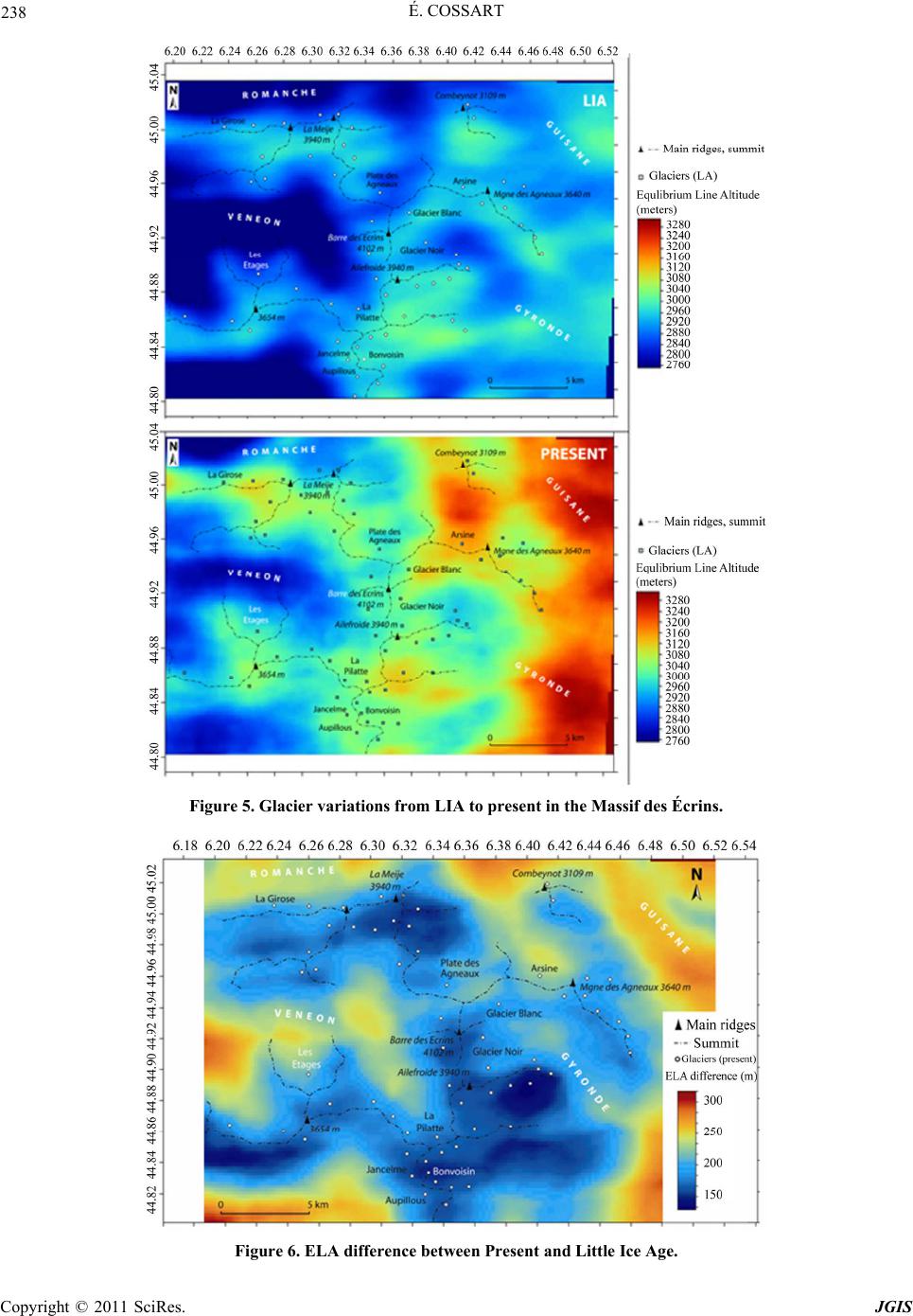

É. COSSART
238
Figure 5. Glacier variations from LIA to present in the Massif des Écrins.
Figure 6. ELA difference between Present and Little Ice Age.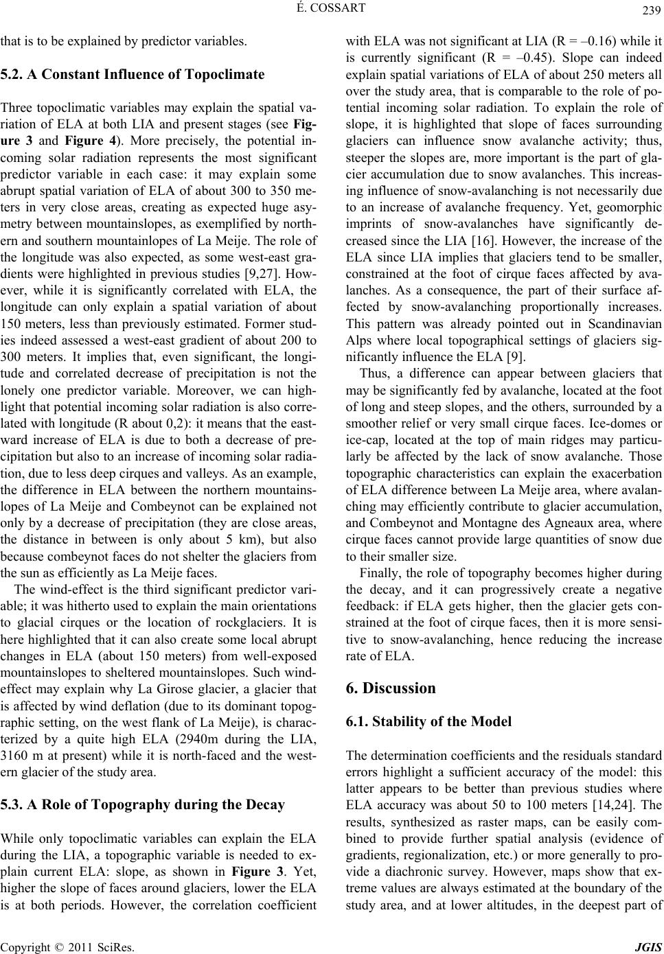

É. COSSART
239
that is to be explained b y predictor variables.
5.2. A Constant Influence of Topoclimate
Three topoclimatic variables may explain the spatial va-
riation of ELA at both LIA and present stages (see Fig-
ure 3 and Figure 4). More precisely, the potential in-
coming solar radiation represents the most significant
predictor variable in each case: it may explain some
abrupt spatial variation of ELA of about 300 to 350 me-
ters in very close areas, creating as expected huge asy-
metry between mountainslopes, as exemplified by north-
ern and southern mountainlopes of La Meije. The role of
the longitude was also expected, as some west-east gra-
dients were highlighted in previous studies [9,27]. How-
ever, while it is significantly correlated with ELA, the
longitude can only explain a spatial variation of about
150 meters, less than previously estimated. Former stud-
ies indeed assessed a west-east gradient of about 200 to
300 meters. It implies that, even significant, the longi-
tude and correlated decrease of precipitation is not the
lonely one predictor variable. Moreover, we can high-
light that potential inco ming solar radiation is also corre-
lated with longitude (R about 0,2 ): it means that the east-
ward increase of ELA is due to both a decrease of pre-
cipitation but also to an increase of incoming solar rad ia-
tion, due to less deep cirques and valleys. As an example,
the difference in ELA between the northern mountains-
lopes of La Meije and Combeynot can be explained not
only by a decrease of precipitation (they are close areas,
the distance in between is only about 5 km), but also
because combeynot faces do not shelter the glaciers from
the sun as efficiently as La Meije faces.
The wind-effect is the third significant predictor vari-
able; it was hitherto used to explain the main orientations
to glacial cirques or the location of rockglaciers. It is
here highlighted that it can also create some local abrupt
changes in ELA (about 150 meters) from well-exposed
mountainslopes to sheltered mountainslopes. Such wind-
effect may explain why La Girose glacier, a glacier that
is affected by wind deflation (due to its domin ant topog-
raphic setting, on the west flank of La Meije), is charac-
terized by a quite high ELA (2940m during the LIA,
3160 m at present) while it is north-faced and the west-
ern glacier of the study area.
5.3. A Role of Topography during the Decay
While only topoclimatic variables can explain the ELA
during the LIA, a topographic variable is needed to ex-
plain current ELA: slope, as shown in Figure 3. Yet,
higher the slope of faces around glaciers, lower the ELA
is at both periods. However, the correlation coefficient
with ELA was not significant at LIA (R = –0.16) while it
is currently significant (R = –0.45). Slope can indeed
explain spatial variations of ELA of abou t 250 meters all
over the study area, that is comparable to the role of po-
tential incoming solar radiation. To explain the role of
slope, it is highlighted that slope of faces surrounding
glaciers can influence snow avalanche activity; thus,
steeper the slopes are, more important is the part of gla-
cier accumulation due to snow avalanches. This increas-
ing influence of snow-avalanching is not necessarily due
to an increase of avalanche frequency. Yet, geomorphic
imprints of snow-avalanches have significantly de-
creased since the LIA [16]. However, the increase of the
ELA since LIA implies that glaciers tend to be smaller,
constrained at the foot of cirque faces affected by ava-
lanches. As a consequence, the part of their surface af-
fected by snow-avalanching proportionally increases.
This pattern was already pointed out in Scandinavian
Alps where local topographical settings of glaciers sig-
nificantly influence the ELA [9].
Thus, a difference can appear between glaciers that
may be significantly fe d by avalanche, located at the foot
of long and steep slopes, and the others, surrounded by a
smoother relief or very small cirque faces. Ice-domes or
ice-cap, located at the top of main ridges may particu-
larly be affected by the lack of snow avalanche. Those
topographic characteristics can explain the exacerbation
of ELA difference between La Meije area, where avalan-
ching may efficiently contribute to glacier accumulation,
and Combeynot and Montagne des Agneaux area, where
cirque faces cannot provide large quantities of snow due
to their smaller size.
Finally, the role of topography becomes higher during
the decay, and it can progressively create a negative
feedback: if ELA gets higher, then the glacier gets con-
strained at the foot of cirque faces, then it is more sensi-
tive to snow-avalanching, hence reducing the increase
rate of ELA.
6. Discussion
6.1. Stability of the Model
The determination coefficients and the residuals standard
errors highlight a sufficient accuracy of the model: this
latter appears to be better than previous studies where
ELA accuracy was about 50 to 100 meters [14,24]. The
results, synthesized as raster maps, can be easily com-
bined to provide further spatial analysis (evidence of
gradients, regionalization, etc.) or more generally to pro-
vide a diachronic survey. However, maps show that ex-
treme values are always estimated at the boundary of the
study area, and at lower altitudes, in the deepest part of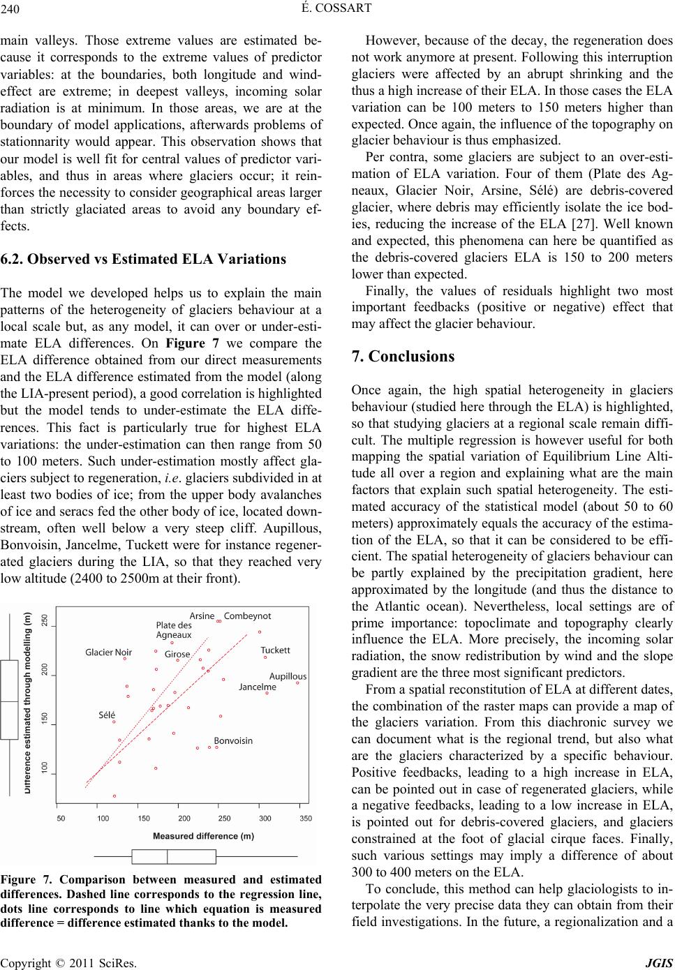

240 É. COSSART
main valleys. Those extreme values are estimated be-
cause it corresponds to the extreme values of predictor
variables: at the boundaries, both longitude and wind-
effect are extreme; in deepest valleys, incoming solar
radiation is at minimum. In those areas, we are at the
boundary of model applications, afterwards problems of
stationnarity would appear. This observation shows that
our model is well fit for central values of predictor vari-
ables, and thus in areas where glaciers occur; it rein-
forces the necessity to consider geographical areas larger
than strictly glaciated areas to avoid any boundary ef-
fects.
6.2. Observed vs Estimated ELA Variations
The model we developed helps us to explain the main
patterns of the heterogeneity of glaciers behaviour at a
local scale but, as any model, it can over or under-esti-
mate ELA differences. On Figure 7 we compare the
ELA difference obtained from our direct measurements
and the ELA difference estimated from the model (along
the LIA-present per iod) , a good co rr elation is h igh ligh ted
but the model tends to under-estimate the ELA diffe-
rences. This fact is particularly true for highest ELA
variations: the under-estimation can then range from 50
to 100 meters. Such under-estimation mostly affect gla-
ciers subject to regeneration, i.e. glaciers subdivided in at
least two bodies of ice; from the upper body avalanches
of ice and seracs fed the other body of ice, located down-
stream, often well below a very steep cliff. Aupillous,
Bonvoisin, Jancelme, Tuckett were for instance regener-
ated glaciers during the LIA, so that they reached very
low altitude (2400 to 2500m at their front).
Figure 7. Comparison between measured and estimated
differences. Dashed line corresponds to the regression line,
dots line corresponds to line which equation is measured
difference = difference estimated thanks to the model.
However, because of the decay, the regeneration does
not work anymore at present. Following this interruption
glaciers were affected by an abrupt shrinking and the
thus a hig h in cr e as e of their ELA. In those cases th e EL A
variation can be 100 meters to 150 meters higher than
expected. Once again, the influence of the topogr aphy on
glacier behaviour is thus emphasized.
Per contra, some glaciers are subject to an over-esti-
mation of ELA variation. Four of them (Plate des Ag-
neaux, Glacier Noir, Arsine, Sélé) are debris-covered
glacier, where debris may efficiently isolate the ice bod-
ies, reducing the increase of the ELA [27]. Well known
and expected, this phenomena can here be quantified as
the debris-covered glaciers ELA is 150 to 200 meters
lower than expected.
Finally, the values of residuals highlight two most
important feedbacks (positive or negative) effect that
may affect the glacier behaviour.
7. Conclusions
Once again, the high spatial heterogeneity in glaciers
behaviour (studied here through the ELA) is highlighted,
so that studying glaciers at a regional scale remain diffi-
cult. The multiple regression is however useful for both
mapping the spatial variation of Equilibrium Line Alti-
tude all over a region and explaining what are the main
factors that explain such spatial heterogeneity. The esti-
mated accuracy of the statistical model (about 50 to 60
meters) approximately equals the accuracy of the estima-
tion of the ELA, so that it can be considered to be effi-
cient. The spatial heterogeneity of glaciers behaviour can
be partly explained by the precipitation gradient, here
approximated by the longitude (and thus the distance to
the Atlantic ocean). Nevertheless, local settings are of
prime importance: topoclimate and topography clearly
influence the ELA. More precisely, the incoming solar
radiation, the snow redistribution by wind and the slope
gradient are the three most significant predictors.
From a spatial reconstitution of ELA at differen t dates,
the combination of the raster maps can provide a map of
the glaciers variation. From this diachronic survey we
can document what is the regional trend, but also what
are the glaciers characterized by a specific behaviour.
Positive feedbacks, leading to a high increase in ELA,
can be pointed out in case of regenerated glaciers, while
a negative feedbacks, leading to a low increase in ELA,
is pointed out for debris-covered glaciers, and glaciers
constrained at the foot of glacial cirque faces. Finally,
such various settings may imply a difference of about
300 to 400 meters on the ELA.
To conclude, this method can help glaciologists to in-
terpolate the very precise d ata they can obtain from their
field investigations. In the futu re, a regionalization and a

É. COSSART
241
classification of glaciers should be planned. Such a re-
gional survey is moreover of prime importance for hy-
drologists that want to assess the consequences of glacier
decay at catchment scales.
8. References
[1] R. Bonaparte, “Variations Périodiques des Glaciers
Français,”Annuaire du Club Alpin Français, Vol. 17,
1890, pp. 425-447.
[2] R. Bonaparte, “Variations Périodiques des Glaciers Fran-
çais,”Annuaire du Club Alpin Français, Vol. 18, No. ,
1891, pp. 482-519.
[3] S.C. Porter, “Present and Past Glaciation Threshold in the
Cascade Range, (Washington, USA),” Journal of Glaci-
ology, Vol. 18, No. 78, 1977, pp. 101-115.
[4] A. Rabatel, J. P. Dedieu and L. Reynaud, “Suivi du Bilan
de Masse Glaciaire Par Télédétection: Application au
Glacier Blanc (Massif des Ecrins, France) Entre 1985 et
2000,” Revue de Géographie Alpine, 2002, pp. 99-109.
doi:10.3406/rga.2002.3094
[5] C. Rabot, “Essai de Chronologie des Variations Gla-
ciaires,” Extrait du Bulletin de Géographie Historique et
Descriptive, Paris, 1902, p. 47.
[6] S.C. Porter, “Equilibrium-Line Altitudes of Late-Quarter-
nary Glaciers in the Southern Alps, New Zealand,” Qua-
ternary Research, Vol. 5, No. , 1975, pp. 27-47.
[7] M. Chenet, E. Roussel, V. Jomelli and D. Grancher,
“Asynchronous Little Ice Age Glacial Maximum Extent
in South-East Iceland,” Geomorphology, Vol. 114, No. 3,
2010, pp. 253-260. doi:10.1016/j.geomorph.2009.07.012
[8] J. L. Edouard, “Les Fluctuations Glaciaires dans le Haut
Bassin de la Romanche,”Ph. D Thesis, Université Gre-
noble I, 1979, p. 685.
[9] D. Six, L. Reynaud and A. Letréguilly, “Bilans de Masse
Des Glaciers Alpins et Scandinaves, Leurs Relations avec
L’oscillation du Climat de L’atlantique Nord,” Comptes
Rendus Académie Sciences, Sciences de la Terre et des
planètes, Vol. 333, 2001, pp. 693-698.
[10] E. Cossart, “Cartographier les Variations Glaciaires,” Le
Monde des Cartes—revue du Comité Français de Carto-
graphie, Vol. 203, 2010, pp. 17-31.
[11] I. S. Evans and N. Cox, “The Form of Glacial Cirques In
the English Lake Disctrict, Cumbria,” Zeitschrift für
Geomorphologie NF, Vol. 43, No. 2, 1995, pp. 203-234.
[12] C. Vincent, “Influence of Climate Change over the 20th
Century on Four French Glacier Mass Bala nces, ” Journal
of Geophysical Research, Vol. 107, No. D19, 2002, pp.
1-12. doi:10.1029/2001JD000832
[13] D. I. Benn and D. J. Evans, “Glaciers and Glaciations,”
Oxford University Press, New York, 1998, p. 734.
[14] J. Ehlers, “Quaternary and Glacial Geology,” John Wiley
and Sons, Chichester, 1996, p. 578.
[15] A. Colas, “Recherches Géomorphologiques en Va-
llouise,” Ph. D Thesis, Lille 1 University, Lille, 2000, p.
291.
[16] V. Jomelli and B. Francou, “Comparing the Characteris-
tics of Rockfall Talus and Snow Avalanche Landforms in
an Alpine Environment Using a New Methodological
Approach (Massif des Ecrins, French Alps),” Geomor-
phology, Vol. 35, No. , 2000, pp. 181-192.
[17] D. I. Benn and A. M. Gemmell, “Calculating Equilib-
rium-Line Altitudes of Former Glaciers by the Balance
Ratio Method: A New Computer Spreadsheet,” Glacial
Geology and Geomorphology, Vol. , No. , 1997, p. 7.
http://ggg.qub.ac.uk/ggg
[18] T. C. Meierding, “Late Pleistocene Equilibrium-Line
Altitudes in the Colorado Front Range: A Comparison of
Methods,” Quaternary Research, Vol. 18, No. , 1982, pp.
289-310.
[19] A. Nesje and S. O. Dahl, “Glaciers and Environmental
Change,” Arnold, London, 2000, p. 347.
[20] J. L. Edouard, “Les Lacs D’Altitude dans les Al pes Fran-
Çaises,”Thesis, Université Grenoble I, Grenoble, 1994, p.
685.
[21] A. Allix, “Les glaciers des Alpes Françaises en 1921”,
Revue de Géographie Alpine, Vol. X, 1922, pp.325-333.
doi:10.3406/rga.1922.1697
[22] A. Allix, “Mémoire sur les observations glaciologiques,
faites en Dauphiné jusqu’en 1924”, Etudes glaciologiques,
Vol. VI, 1924, pp. 1-138.
[23] R. Blanchard, “La Crue Glaciaire dans les Alpes de
Savoie au XVIIè Siècle”, Revue de Géographie Alpine,
Vol. 1, 1913, pp. 443-454.
[24] J. L. Carrivick and T. R. Brewer, “Improving Local Esti-
Mations and Regional Trends of Glacier Equilibrium
Line Altitudes,” Geografiska Annaler: Series A, Physical
Geography, Vol. 86, No. 1, March 2004, pp. 67-79.
doi:10.1111/j.0435-3676.2004.00214.x
[25] D. Burbank and M. Fort, “Bedrock Control on Glacial
Limits: Examples of the Ladakh and Zanskar Ranges,
North-Western Himalaya, India,” Journal of Glaciology,
Vol. 31, No. 108, 1985, pp. 143-149.
[26] E. Cossart, Y. Drocourt and B. Anselme, “Variations
Gla-ciaires Dans les Andes de Mendoza Entre 1975 et
2007,” M@ppemonde, Vol. 97, 2010.
http://mappemonde.mgm.fr/num25/articles/art10103.html
[27] R. Vivian, “Les Glaciers des Alpes Occidentales,” Thesis,
Université Joseph Fourier-Grenoble I, Grenoble, 1975, p.
470.
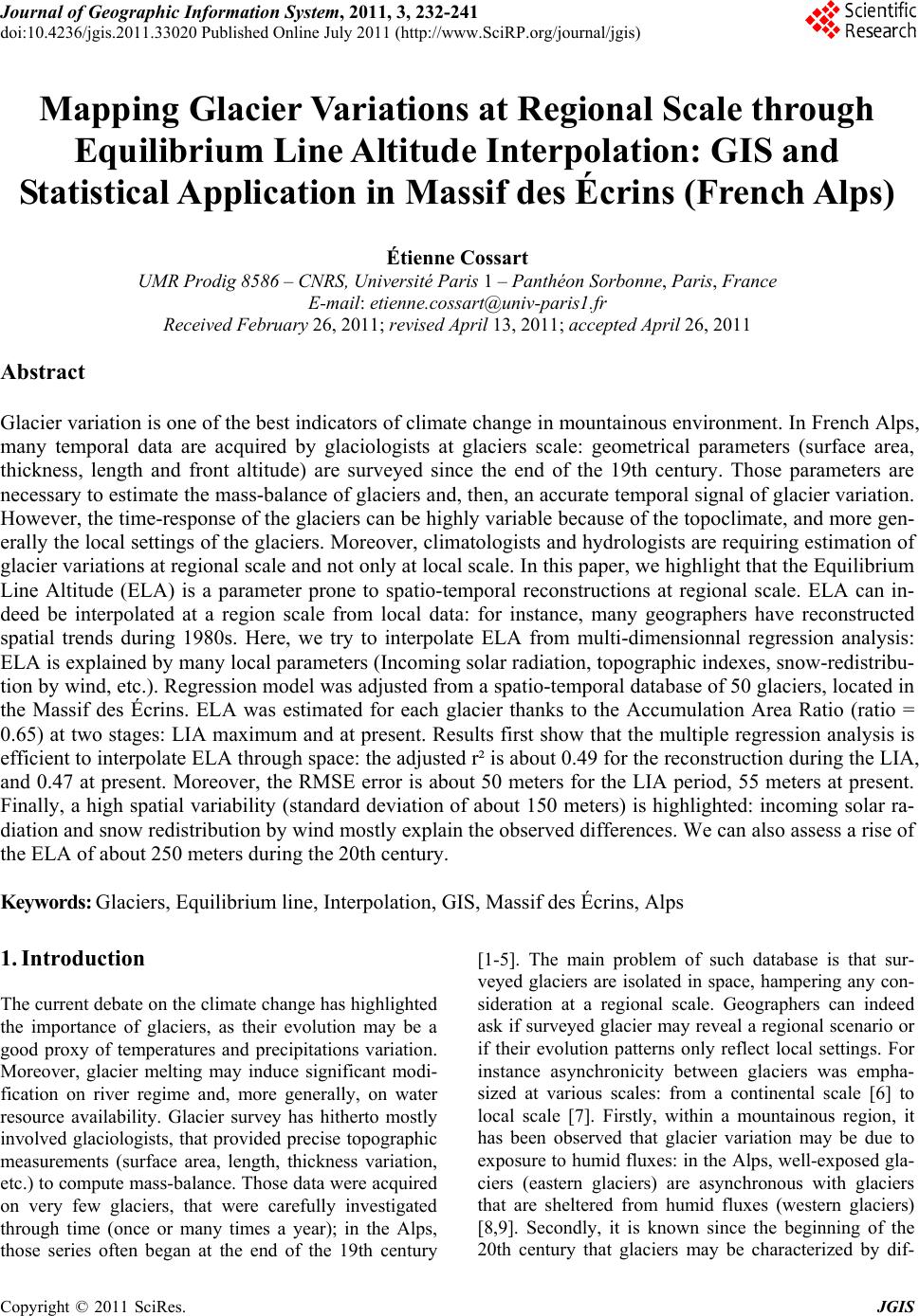