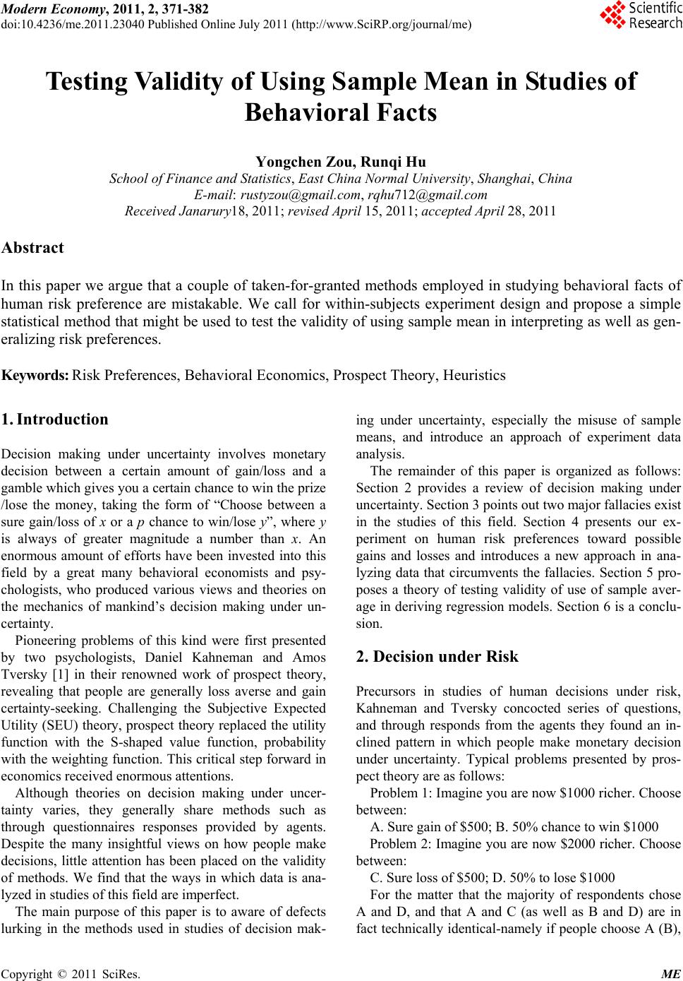Modern Economy, 2011, 2, 371-382
doi:10.4236/me.2011.23040 Published Online July 2011 (http://www.SciRP.org/journal/me)
Testing Validity of Using Sample Mean in Studies of
Behavioral Facts
Yongchen Zou, Runqi Hu
School of Finance and St at i stics, East China Normal University, Shanghai, China
Received Janarury18, 2011; revised April 15, 2011; accepted April 28, 2011
Abstract
In this paper we argue that a couple of taken-for-granted methods employed in studying behavioral facts of
human risk preference are mistakable. We call for within-subjects experiment design and propose a simple
statistical method that might be used to test the validity of using sample mean in interpreting as well as gen-
eralizing risk preferences.
Keywords: Risk Preferences, Behavioral Economics, Prospect Theory, Heuristics
1. Introduction
Decision making under uncertainty involves monetary
decision between a certain amount of gain/loss and a
gamble which gives you a certain chance to win the prize
/lose the money, taking the form of “Choose between a
sure gain/loss of x or a p chance to win/lose y”, where y
is always of greater magnitude a number than x. An
enormous amount of efforts have been invested into this
field by a great many behavioral economists and psy-
chologists, who produced various views and theories on
the mechanics of mankind’s decision making under un-
certainty.
Pioneering problems of this kind were first presented
by two psychologists, Daniel Kahneman and Amos
Tversky [1] in their renowned work of prospect theory,
revealing that people are generally loss averse and gain
certainty-seeking. Challenging the Subjective Expected
Utility (SEU) theory, prospect theory replaced the utility
function with the S-shaped value function, probability
with the weighting function. This critical step forward in
economics received enormous attentions.
Although theories on decision making under uncer-
tainty varies, they generally share methods such as
through questionnaires responses provided by agents.
Despite the many insightful views on how people make
decisions, little attention has been placed on the validity
of methods. We find that the ways in which data is ana-
lyzed in studies of this field are imperfect.
The main purpose of this paper is to aware of defects
lurking in the methods used in studies of decision mak-
ing under uncertainty, especially the misuse of sample
means, and introduce an approach of experiment data
analysis.
The remainder of this paper is organized as follows:
Section 2 provides a review of decision making under
uncertainty. Section 3 points out two major fallacies exist
in the studies of this field. Section 4 presents our ex-
periment on human risk preferences toward possible
gains and losses and introduces a new approach in ana-
lyzing data that circumvents the fallacies. Section 5 pro-
poses a theory of testing validity of use of sample aver-
age in deriving regression models. Section 6 is a conclu-
sion.
2. Decision under Risk
Precursors in studies of human decisions under risk,
Kahneman and Tversky concocted series of questions,
and through responds from the agents they found an in-
clined pattern in which people make monetary decision
under uncertainty. Typical problems presented by pros-
pect theory are as follows:
Problem 1: Imagine you are now $1000 richer. Choose
between:
A. Sure gain of $500; B. 50% chance to win $1000
Problem 2: Imagine you are now $2000 richer. Choose
between:
C. Sure loss of $500; D. 50% to lose $1000
For the matter that the majority of respondents chose
A and D, and that A and C (as well as B and D) are in
fact technically identical-namely if people choose A (B),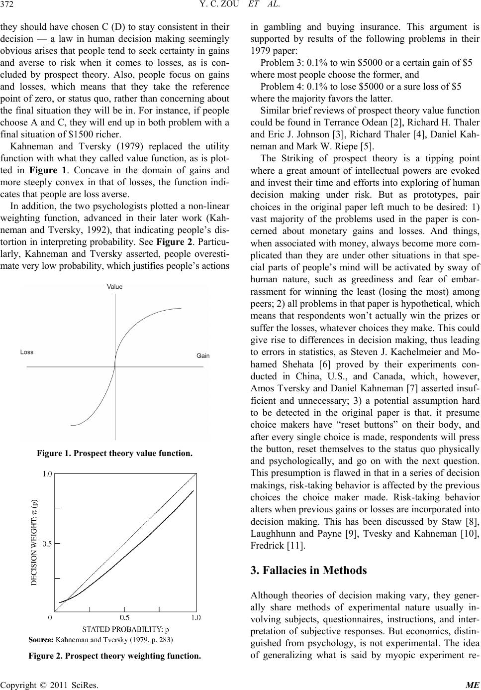

Y. C. ZOU ET AL. 372
they should have chosen C (D) to stay consistent in their
decision — a law in human decision making seemingly
obvious arises that people tend to seek certainty in gains
and averse to risk when it comes to losses, as is con-
cluded by prospect theory. Also, people focus on gains
and losses, which means that they take the reference
point of zero, or status quo, rather than concerning about
the final situation they will be in. For instance, if people
choose A and C, they will end up in both problem with a
final situation of $1500 richer.
Kahneman and Tversky (1979) replaced the utility
function with what they called value function, as is plot-
ted in Figure 1. Concave in the domain of gains and
more steeply convex in that of losses, the function indi-
cates that people are loss averse.
In addition, the two psychologists plotted a non-linear
weighting function, advanced in their later work (Kah-
neman and Tversky, 1992), that indicating people’s dis-
tortion in interpreting probability. See Figure 2. Particu-
larly, Kahneman and Tversky asserted, people overesti-
mate very low probability, which justifies people’s actions
Figure 1. Prospect theory value function.
Figure 2. Prospect theory weighting function.
in gambling and buying insurance. This argument is
supported by results of the following problems in their
1979 paper:
Problem 3: 0.1% to win $5000 or a certain gain of $5
where most people choose the former, and
Problem 4: 0.1% to lose $5000 or a sure loss of $5
where the majority favors the latter.
Similar brief reviews of prospect theory value function
could be found in Terrance Odean [2], Richard H. Thaler
and Eric J. Johnson [3], Richard Thaler [4], Daniel Kah-
neman and Mark W. Riepe [5].
The Striking of prospect theory is a tipping point
where a great amount of intellectual powers are evoked
and invest their time and efforts into exploring of human
decision making under risk. But as prototypes, pair
choices in the original paper left much to be desired: 1)
vast majority of the problems used in the paper is con-
cerned about monetary gains and losses. And things,
when associated with money, always become more com-
plicated than they are under other situations in that spe-
cial parts of people’s mind will be activated by sway of
human nature, such as greediness and fear of embar-
rassment for winning the least (losing the most) among
peers; 2) all problems in that paper is hypothetical, which
means that respondents won’t actually win the prizes or
suffer the losses, whatever choices they make. This could
give rise to differences in decision making, thus leading
to errors in statistics, as Steven J. Kachelmeier and Mo-
hamed Shehata [6] proved by their experiments con-
ducted in China, U.S., and Canada, which, however,
Amos Tversky and Daniel Kahneman [7] asserted insuf-
ficient and unnecessary; 3) a potential assumption hard
to be detected in the original paper is that, it presume
choice makers have “reset buttons” on their body, and
after every single choice is made, respondents will press
the button, reset themselves to the status quo physically
and psychologically, and go on with the next question.
This presumption is flawed in that in a series of decision
makings, risk-taking behavior is affected by the previous
choices the choice maker made. Risk-taking behavior
alters when previous gains or losses are incorporated into
decision making. This has been discussed by Staw [8],
Laughhunn and Payne [9], Tvesky and Kahneman [10],
Fredrick [11].
3. Fallacies in Methods
Although theories of decision making vary, they gener-
ally share methods of experimental nature usually in-
volving subjects, questionnaires, instructions, and inter-
pretation of subjective responses. But economics, distin-
guished from psychology, is not experimental. The idea
of generalizing what is said by myopic experiment re-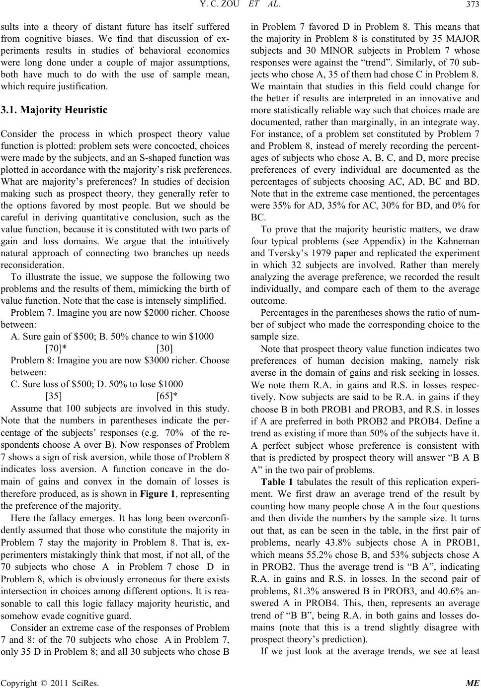

Y. C. ZOU ET AL.373
sults into a theory of distant future has itself suffered
from cognitive biases. We find that discussion of ex-
periments results in studies of behavioral economics
were long done under a couple of major assumptions,
both have much to do with the use of sample mean,
which require justification.
3.1. Majority Heuristic
Consider the process in which prospect theory value
function is plotted: problem sets were concocted, choices
were made by the subjects, and an S-shaped function was
plotted in accordance with the majority’s risk preferences.
What are majority’s preferences? In studies of decision
making such as prospect theory, they generally refer to
the options favored by most people. But we should be
careful in deriving quantitative conclusion, such as the
value function, because it is constituted with two parts of
gain and loss domains. We argue that the intuitively
natural approach of connecting two branches up needs
reconsideration.
To illustrate the issue, we suppose the following two
problems and the results of them, mimicking the birth of
value function. Note that the case is intensely simplified.
Problem 7. Imagine you are now $2000 richer. Choose
between:
A. Sure gain of $500; B. 50% chance to win $1000
[70]* [30]
Problem 8: Imagine you are now $3000 richer. Choose
between:
C. Sure loss of $500; D. 50% to lose $1000
[35] [65]*
Assume that 100 subjects are involved in this study.
Note that the numbers in parentheses indicate the per-
centage of the subjects’ responses (e.g. of the re-
spondents choose A over B). Now responses of Problem
7 shows a sign of risk aversion, while those of Problem 8
indicates loss aversion. A function concave in the do-
main of gains and convex in the domain of losses is
therefore produced, as is shown in Figure 1, representing
the preference of the majority.
70%
Here the fallacy emerges. It has long been overconfi-
dently assumed that those who constitute the majority in
Problem 7 stay the majority in Problem 8. That is, ex-
perimenters mistakingly think that most, if not all, of the
70 subjects who chose in Problem 7 chose in
Problem 8, which is obviously erroneous for there exists
intersection in choices among different options. It is rea-
sonable to call this logic fallacy majority heuristic, and
somehow evade cognitive guard.
A D
Consider an extreme case of the responses of Problem
7 and 8: of the 70 subjects who chose in Problem 7,
only 35 D in Problem 8; and all 30 subjects who chose B
in Problem 7 favored D in Problem 8. This means that
the majority in Problem 8 is constituted by 35 MAJOR
subjects and 30 MINOR subjects in Problem 7 whose
responses were against the “trend”. Similarly, of 70 sub-
jects who chose A, 35 of them had chose C in Problem 8.
A
We maintain that studies in this field could change for
the better if results are interpreted in an innovative and
more statistically reliable way such that choices made are
documented, rather than marginally, in an integrate way.
For instance, of a problem set constituted by Problem 7
and Problem 8, instead of merely recording the percent-
ages of subjects who chose A, B, C, and D, more precise
preferences of every individual are documented as the
percentages of subjects choosing AC, AD, BC and BD.
Note that in the extreme case mentioned, the percentages
were 35% for AD, 35% for AC, 30% for BD, and 0% for
BC.
To prove that the majority heuristic matters, we draw
four typical problems (see Appendix) in the Kahneman
and Tversky’s 1979 paper and replicated the experiment
in which 32 subjects are involved. Rather than merely
analyzing the average preference, we recorded the result
individually, and compare each of them to the average
outcome.
Percentages in the parentheses shows the ratio of num-
ber of subject who made the corresponding choice to the
sample size.
Note that prospect theory value function indicates two
preferences of human decision making, namely risk
averse in the domain of gains and risk seeking in losses.
We note them R.A. in gains and R.S. in losses respec-
tively. Now subjects are said to be R.A. in gains if they
choose B in both PROB1 and PROB3, and R.S. in losses
if A are preferred in both PROB2 and PROB4. Define a
trend as existing if more than 50% of the subjects have it.
A perfect subject whose preference is consistent with
that is predicted by prospect theory will answer “B A B
A” in the two pair of problems.
Table 1 tabulates the result of this replication experi-
ment. We first draw an average trend of the result by
counting how many people chose A in the four questions
and then divide the numbers by the sample size. It turns
out that, as can be seen in the table, in the first pair of
problems, nearly 43.8% subjects chose A in PROB1,
which means 55.2% chose B, and 53% subjects chose A
in PROB2. Thus the average trend is “B A”, indicating
R.A. in gains and R.S. in losses. In the second pair of
problems, 81.3% answered B in PROB3, and 40.6% an-
swered A in PROB4. This, then, represents an average
trend of “B B”, being R.A. in both gains and losses do-
mains (note that this is a trend slightly disagree with
prospect theory’s prediction).
If we just look at the average trends, we see at least

Y. C. ZOU ET AL. 374
Table 1. Result of a replication experiment of four prospect
theory problems.
Subject PROB1 PROB2 PROB3 PROB4
1 B A B A
2 A B B A
3 B A B B
4 B B B B
5 B A B B
6 A A B A
7 A A B A
8 B A B B
9 A A B B
10 A B B B
11 A B A B
12 A B A B
13 A A B B
14 B B A B
15 B A B A
16 B A B A
17 B B A A
18 B B B A
19 B B B A
20 B A B A
21 B B B B
22 A A B B
23 B B B B
24 A B B B
25 B A B A
26 A A B B
27 A A A B
28 A B B B
29 B B B B
30 B A A B
31 A B B A
32 B A B A
Choose A 14 [43.75%] 17 [53.13%] 6 [18.75%] 13 [40.63%]
Choose BA 10 [31.25%] 12 [37.5%]
Choose
BA,BA 6 [18.75%]
one of them is consistent with S-shaped value function,
and one might argue that if the sample size (or the num-
ber of questions) expands, prospect theory prediction
could be proved right. However, if the result of this rep-
lication experiment is interpreted in a different way, the
conclusion would be widely contradicting.
Instead of calculating an average answer, we now look
at within-subjects, or integrate, results by checking how
many subjects answered “B A” in both pair of questions,
and recall that “B A” indicates a preference of R. A. in
gains and R.S. in losses. As is shown in Table 1, only
31.3% and 37.5% of subjects answered “B A” in the
pairs of questions respectively, a result far cry in indi-
cating the trend of R.A. in gains and R.S. in losses. And
the majority heuristic is proved existing here because
although the average result shows a trend of R.A. and
R.S. in the first pair of questions, it is actually supported
by only 31.3% of the subjects.
Remarkably, this paradox becomes more irony when
we try to find “perfect subject” who answered “B A B
A”: there are only six of them, namely 18.8% of the
sample. If a trend is buttressed by no more than 20% of
the subjects, it can never be called a trend.
We argue that the majority heuristic has taught us a
paradoxical lesson that, people might be risk averse in
gains; people might be risk seeking in losses; but it
would be erroneous to assert that people are risk averse
in gains and risk seeking in losses. As a matter of fact,
we are to show in section III that even in the domains of
gains and losses respectively, human preferences cannot
be simply generalized as risk averse or risk seeking.
We should however point out that intersection of pref-
erences doesn’t happen all the time. Think of another
two problems and a pair of possible results:
Problem 9. Choose between:
A. Sure gain of $500; B. 50% chance to win $1000
[70]* [30]
Problem 10: Choose between:
C. Sure gain of $600; D. 50% chance to win $1,000
[75]* [25]
It is reasonable in this case to predict that all those
who chose A in the former problem favored C in the lat-
ter — no intersection happens. We speculate two pairs of
principles in human preferences here. Suppose A and B
are two outcomes,

a positive amount, and p a prob-
ability that 0p1

, then
a) If A is preferred to pB, A

 is preferred to pB;
but A


is not necessarily preferred to BpP





;
b) If pB is preferred to A,

Bp


 is preferred to A;
but


Bp


is not necessarily preferred to Ap


.
This indicates that an increment of benefit on the op-
tion favored would firm up the chooser’s preference,

Y. C. ZOU ET AL.375
while increments on both sides don’t.
3.2. Misuse of Sample Mean
Studies that use statistical methods require appropriate
understanding of statistics used. When we require sub-
jective certainty equivalents for lotteries out of subjects,
we must make sure that the subjects understand what
mathematical expectation is because it would be unfair
otherwise to use the statistic that subjects don’t under-
stand later as a criterion testing subjects’ preferences.
More importantly, we should sure that we experimenters
ourselves fully understand the statistics we are using.
However, there exists the logic leap from existence of
statistic to apprehension of statistic. Just the fact that the
statistics are invented doesn’t mean they could be fully
understood. Typical example here is, we are of the opin-
ion, the basic and long been misused statistic of average.
Average, arithmetic or compound, is a basic statistic
that is used everywhere as a estimator of general stan-
dard. Broadly as it has long been used, human mind
could hardly grasp what an average really is. When it is
said that Class A bares an average score of 75 in a
mid-term examination, it is interpreted immediately by
human mind, or at least System 1, that almost every stu-
dent in Class A got test results in the neighborhood of 75,
which is obviously erroneous. And when the second
news came that Class B has an average score of 82, again
it is translated into a statement that almost every student
in Class B got a better score than students in Class A.
Ludicrous as it may sound, and despite almost everyone
would deny these kinds of thoughts had ever come to
them and they really understand what is an average, the
very logical fallacy is repeated frequently in studies of
human preferences, especially in those which experi-
ments involving subjects are conducted.
The common use of average is like this: conduct the
experiment to the subjects, have their responses docu-
mented, average the answers and analyze the average
answer as a supposed individual who represents the
whole sample. The basic idea of using average is to av-
erage out unwelcome volatility and thus get a general
trend. But this could be perilous in studying behavioral
facts of human preferences, for in these kinds of studies,
what we need is exactly the opposite: human preferences,
such as risk preferences, are very volatile, to say nothing
of the fact that an individual’s preference vary under
arbitrary situations. And this very divergence in prefer-
ences is exactly what worth investigating. This is not to
say average should be abandoned in preferences analysis.
As a matter of fact, one can never avoid using it because
it would be invalid and unnecessary to focus on every
individual. However, we can revise the sample mean
method by dividing the whole sample into groups with
obviously different characteristics, thus saving these di-
vergences from being willy-nilly averaged out. We are to
employ this method into our experiment in Part III.
Failure of human minds’ apprehension of other statis-
tics, such as expected value are entertainingly discussed
by Taleb [12], where he asked readers to imagine a com-
bination of pleasure of a vacation that will happen 85%
in Paris and 15% in Caribbean. In fact, he asserted, that
“[our] brain can properly handle one and only one state
at once — unless [you] have personality troubles of a
deeply pathological nature”.
4. Risk Preference Families
So far we have shown that the linkage of the two
branches of the value function and the use of total aver-
age in studying human preferences are mistakable. And
we claimed in Section II that not only risk preferences
should be studied separately in gain and loss domain,
even in the domains of gain or loss per se, they cannot be
simply generalized as “risk averse” or “risk seeking”.
Our experiment following is to test the different risk
preferences under gambles of different prize level.
4.1. The Experiment and Results
The process employed a two-stage method proved unbi-
ased by Becker et al. [13]. But rather than eliciting sub-
jective certainty equivalents under different probability
to win, we require certainty equivalents under different
prizes and losses at a same probability 50%. Prizes and
losses provided in the experiment ranged from 2 to
1000000 (2, 6, 10, 15, 25, 30, 50, 100, 200, 400, 750,
1000, 5000, 100000, 1000000). The experimental in-
structions are written in English. We assume this to be a
semi-“back translation” (a concept put forward by Brislin
[14]) for we, the designers, are Chinese).
The reason why we didn’t divide the probability into
smaller minor unity is that we fear that gradual increases
in probability make people confused and thus inducing
mindless answers. We assume that people get vague idea
about the difference between chances of 30% and 40%,
but they surely feel different among a half chance to win,
less than a half to win, and more than a half to win.
Hence we choose 50% as our constant probability, pre-
suming that our subjects stay cognitively conscious dur-
ing the test.
Note that all subjects are students major in either sta-
tistics, actuarial science, risk management, or financial
engineering, hence it is reasonable to assume than they
know quite well the concept of mathematical expectation,
justifying our using it later as a criterion in discussing

Y. C. ZOU ET AL. 376
risk preferences.
To rule out the majority heuristic and the misuse of
total average discussed in Part II, we employ a different
method in interpreting the results. Risk preferences to-
ward possible gains and losses are discussed separately.
We are to show the risk preferences of gain domain and
those of loss domain, but we don’t and cannot provide a
single type of risk preference that summarizes the whole
picture. We avoid believing in average of the total.
Rather, responses are categorized, according to their
characteristics, into groups. In fact, we intuitively ex-
pected, rather than predicting, a general but nothing spe-
cific trend before we get the results: respondents may
show a tendency toward risk seeking when the possible
prizes/losses are small, and they may tend to be risk
averse when the possible prizes/losses surge to certain
higher levels. However, we didn’t plan to derive the
general trend which represents the average (and we don’t
believe any single one could represents all); instead, we
focus on detecting different patterns of risk preferences
among subjects. We even tried to analyze anomalies
among the results and explain why they are like that.
Defects in our experiment is that it provided no real
money rewards. Since we are trying to elicit subjects’
preference under big prize, we cannot afford to actually
pay them what they won (For experiment that involving
real subjects losses, see Etchart-Vincent and l’Haridon
[15]). But they are informed that rewards are to be paid
according to their final results. Subjects are urged to be-
have as if the gambles are real and independent
throughout the experiment.
We used in the gain domain the ratio of certainty
equivalent to expected value, or CE/E, as major criterion
of subjects risk preferences. If CE/E of a single response
exceeds unity, the subject is said to show a sign of risk
seeking toward the gamble, while if CE/E is lower than
one, it signals risk averse. In the loss domain, on the
other hand, the ratio of maximum premium (which means
that the maximum certain quantity the subject is willing
to pay to eliminate the risk of suffering potential loss) to
expected value, or MP/E, is used so that if MP/E of a
response toward a gamble exceeds one, it shows risk averse,
and if MP/E is less than one, it shows risk seeking. For
example, if the subject is extremely risk seeking toward a
potential loss, then she is not willing to pay even a penny
to an insurer to have her asset underwritten. In this case,
the maximum premium will be 0, thus MP/E is equal to 0.
For the purpose of illustrating the misuse of total av-
erage that has been discussed in Part II, Figure 3 mani-
fests the total average CE/E and MP/E values under the
prize/loss series toward gains and losses respectively. It
seems obvious, from the graphs, that there is a trend of
decreasing CE/E ratio and increasing MP/E ratio. What’s
Figure 3. Total average of CE/E ratio and MP/E ratio.
more, average CE/E ratio of our experiment rarely ex-
ceeds unity conspicuously and so does MP/E ratio. This
indicates that except for extremely small prizes (such as
50% to win 2) and extremely big losses (such as 50% to
lose 1000000), respondents show preferences of risk
averse in gain domain and risk seeking in loss domain,
consistent with what is told by prospect theory and its
value function.
We categorized according to their features the final
results of gain domain and loss domain respectively into
three families. As is shown by Figure 4 some typical
individual responses, these categories are named “Gen-
eral”, “Arch”, and “Bounce” in gains, and “General”,
“Neutral” and “Seeking” in the losses. Do notice that
these results are not paired with each other and must be
viewed separately, which means that, for instance, a
subject in “General” family of gain domain can either be
in “General”, “Neutral” or “Seeking” in the loss part.
The first three captures of Figure 4 manifests three
preference families that we detected from the subjects in
questions involving possible gains. “General” family
shows a preference pattern that fits the majority of the
respondents, in which agents show risk seeking toward
relatively small prizes, and they gradually become risk
averse as the prize become more and more attractive.
Note that although “General”, like the total average CE/E,
decreases as the prize level sour, the line does not fall
below unity until the prize level reaches somewhere
around 200, whereas the total average CE/E rarely sur-
passes one. Respondents in “Arch” family typically start
from strict risk averse, then becomes increasingly risk
seeking, but when the prize level seems attractive enough
to them, they show a sign of risk averse again. The CE/E

Y. C. ZOU ET AL. 377
Figure 4. Categorizing of final results in gain and loss domains.(1.General)
line of this family crosses the unity twice. Subjects in
“Bounce” family, albeit not large in number, shows an
interesting and sharp risk preference reversal when the
prize level gets extremely high, before which they gener-
ally share risk preferences with those in “General” family.
The last three captures, on the other hand, shows the
three risk preference families of the loss domain. Agents
in “General (Loss)” family are shown to have increasing
MP/E ratio as the loss level approaches extreme. But
note that MP/E values of a typical respondent in “Gen-
eral (Loss)” family exceeds unity when the possible loss
level reaches 200 or so, while in total average ratios,
MP/E only goes beyond 1 when the possible loss be-
comes astronomical. “Neutral” family possesses MP/E
ratio hovering around one whatever the possible loss
would be. Finally, subjects in “Seeking” family have
MP/E ratio always below unity; they are always risk
seeking, tending to run the risk of losing.
Counterintuitive finding of our experiment is that risk
preferences of gain and loss domains barely cross paths.
For example, not a single one of the subjects showed a
sign of risk neutral in gains part, and no one in losses
part presented a sudden preference reversal as is in
“Bounce” family. We find that subjects behaved sharply
different toward risks of certain gains and losses, and
their psychologies, influenced by various factors, varied
individually and were very volatile.
We interviewed after the experiment some of the sub-
jects and asked for what were their psychologies when
providing answers. To our surprise, every subject inter-
viewed gave exactly the same reason justifying their
subjective certainty equivalent toward small prized and
losses (such as a 50% to win/lose 2), which goes like:
The possible gains/losses are so small that I don’t care if
I win or lose them. But their explanations diverse. For
those who have CE/E ratio of 2 or bigger toward possible
gain, their explanations were typically “I don’t care
about the little gain so that I just gamble. Either win or
not win, no big deal”; for those who have CE/E ratio of
smaller value, their justifications were like “I don’t care
the winning of the little amount of money”. In the loss
part, none of the subjects has high MP/E ratio toward
small possible loss; they chorused a preference of risk
seeking, with MP/E ratios ranging from 0 to 1. Similarly,
they asserted in the aftermath interview that they “an-
swered so because they didn’t care about the small

Y. C. ZOU ET AL. 378
losses”. Rationally speaking, if subjects “don’t care”
whether they gamble or not, namely they think them-
selves indifferent between gambling or not gambling,
that should be interpreted as risk neutral thus their sub-
jective certainty equivalent should be equal to the
mathematical expectation, entailing a CE/E or MP/E
ratio of 1. However, the data just showed that behavior
of most subjects wasn’t consistent with this rationality.
Thus we have reason to doubt that when CE/E or MP/E
ratio does equal to unity, that doesn’t necessarily mean
the subjects are risk neutral toward the gamble.
The sudden CE/E ratio bounce back of subjects in
“Bounce” family reflects gambler’s psychology. When
respondents in the family were asked why they suddenly
wanted to take risk in the high prize gamble, they typi-
cally answer that when the prize level became extremely
high, the lottery turns into a gamble. And a gamble is a
gamble, either one win the big, or walk away with noth-
ing.
Most subjects in “Neutral” family of loss domain said
they feel horrible on the thought of losing their money,
be it the premium they pay or the money they lose if they
choose to gamble. Rather than endless dithery, they sim-
ply chose to stay indifferent: write down certainty
equivalents entered around mathematical expectations,
and whatever happens is destiny.
Agents in “Seeking” family of loss domain usually
assert that they would rather run the risk of losing the
gamble than paying anything to eradicate the risk, so that
their fortunes still have a good 50% chance to stay intact.
Although we highly doubt that this kind of psychology is
resulted partly from the fact that the possible losses in
the experiment are hypothetical.
4.2. Models
Kachelmeier and Shehata (1992) introduced a linear re-
gression model that includes subject effects, incorporat-
ing correlated errors entailed by individual differences in
risk preferences. Our models bases essentially on the
Kachelmeier and Shehata’s CERATIO model but a) we
ignore the percent effects for lotteries in our experiment
share the constant winning/losing chance of 50%, b) we
used logarithm of prizes/losses in the model and c) we
introduce a similar MPRATIO model for MP/E ratios
with logarithm of prize factor replaced by logarithm of
loss. Our regression models are shown as followed:

1
1
2
1
CERATIOlog Prize
n
jj
jSubject







 (1)

**
1*
2
1
CERATIOlogLoss
i
n
jj
jSubject







 (2)
where CERATIO and MPRATIO respectively means
ratio of certainty equivalent to expected value and ratio
of maximum premium to expected value;

and *

are intercepts of regressions; log(Prize) and log(Loss) are
logarithm of Prizes and Losses series in the lotteries;
j
Su
n
bject refers to subjects factor, which equals 1 if the
observation is from the j th observation, –1 if from the
th observation, and 0 otherwise;

is the disturbance.
The regression coefficients and the results of tests are
tabulated as follows.
Where CONSTANT= the intercept parameter;
i
S
*
p = the j th subject = logarithm of Prize
Advantage of categorizing risk preference into fami-
lies, and thus deriving the categorized regression models,
could be observed first in terms of the increase in both R
square, namely the goodness of fit, and adjusted R square
in both “General” families of gain and loss parts as is
shown by Table 3 and Table 7, compared to that of the
sample average data in Table 2 and Table 6. R square
increases from 0.433 in sample average to 0.758 in
“General” family of gain domain, and from 0.784 in
sample average to 0.839 in “General” family of loss do-
main. And the corresponding adjusted R square as well
increase from 0.392 to 0.533 and from 0.586 to 0.683
respectively. Besides, estimates derived by OLS tech-
nique in CERATIO and MPRATIO model show statisti-
cal significance by and large, as can be seen particularly
in Table 3, Table 5, Table 7, and Table 8. Table 4 and
Table 9, corresponding to “Arch” family of Gain Do-
main and “Seeking” Family of Loss Domain, show in-
significance in estimates of parameters; we attribute this
insignificance to the small sample size, and it can be that
they are not representative to the population.
Second, in most families, the variances of estimates of
both CERATIO and MPRATIO drop from original vari-
ances of estimates of CERATIO and MPRATIO in sam-
ple average regression models, indicating better stability.
See Table 10.
5. “D” for Testing Validity of Sample
Average
It is mentioned without evidence in Sec II.C that the use
of total average in analyzing behavioral facts of human
preferences is mistakable for it averages out not only
unwelcome volatility of the data but also the divergence
between subjects preferences which worth investigating.
This is observable from Figure 3 and Figure 4, espe-
cially in the gain part, for the three risk preference fami-
lies, “General”, “Arch”, and “Bounce”, viz., of gain do-
main bear sharply different shaped CE/E lines.
To test whether the use of sample average averages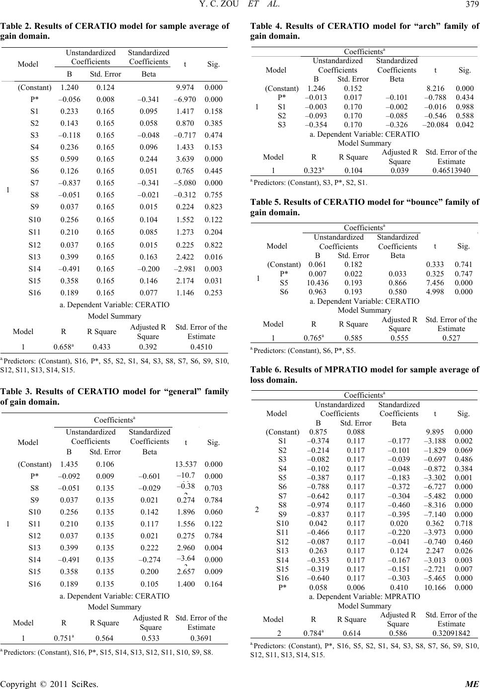

Y. C. ZOU ET AL.379
Table 2. Results of CERATIO model for sample average of
gain domain.
Unstandardized
Coefficients
Standardized
Coefficients
Model
B Std. ErrorBeta
t Sig.
(Constant) 1.240 0.124 9.974 0.000
P* –0.056 0.008 –0.341 –6.9700.000
S1 0.233 0.165 0.095 1.4170.158
S2 0.143 0.165 0.058 0.8700.385
S3 –0.118 0.165 –0.048 –0.7170.474
S4 0.236 0.165 0.096 1.4330.153
S5 0.599 0.165 0.244 3.6390.000
S6 0.126 0.165 0.051 0.7650.445
S7 –0.837 0.165 –0.341 –5.0800.000
S8 –0.051 0.165 –0.021 –0.3120.755
S9 0.037 0.165 0.015 0.2240.823
S10 0.256 0.165 0.104 1.5520.122
S11 0.210 0.165 0.085 1.2730.204
S12 0.037 0.165 0.015 0.2250.822
S13 0.399 0.165 0.163 2.4220.016
S14 –0.491 0.165 –0.200 –2.9810.003
S15 0.358 0.165 0.146 2.1740.031
1
S16 0.189 0.165 0.077 1.1460.253
a. Dependent Variable: CERATIO
Model Summary
Model R R Square Adjusted R
Square
Std. Error of the
Estimate
1 0.658a 0.433 0.392 0.4510
a.Predictors: (Constant), S16, P*, S5, S2, S1, S4, S3, S8, S7, S6, S9, S10,
S12, S11, S13, S14, S15.
Table 3. Results of CERATIO model for “general” family
of gain domain.
Coefficientsa
Unstandardized
Coefficients
Standardized
Coefficients
Model
B Std. ErrorBeta
t Sig.
(Constant) 1.435 0.106 13.537 0.000
P* –0.092 0.009 –0.601 –10.7
32
0.000
S8 –0.051 0.135 –0.029 –0.38
2
0.703
S9 0.037 0.135 0.021 0.2740.784
S10 0.256 0.135 0.142 1.8960.060
S11 0.210 0.135 0.117 1.5560.122
S12 0.037 0.135 0.021 0.2750.784
S13 0.399 0.135 0.222 2.9600.004
S14 –0.491 0.135 –0.274 –3.64
3
0.000
S15 0.358 0.135 0.200 2.6570.009
1
S16 0.189 0.135 0.105 1.4000.164
a. Dependent Variable: CERATIO
Model Summary
Model R R SquareAdjusted R
Square
Std. Error of the
Estimate
1 0.751a 0.564 0.533 0.3691
a.Predictors: (Constant), S16, P*, S15, S14, S13, S12, S11, S10, S9, S8.
Table 4. Results of CERATIO model for “arch” family of
gain domain.
Coefficientsa
Unstandardized
Coefficients
Standardized
Coefficients
Model
B Std. Error Beta
t Sig.
(Constant) 1.2460.152 8.216 0.000
P* –0.0130.017 –0.101 –0.7880.434
S1 –0.0030.170 –0.002 –0.0160.988
S2 –0.0930.170 –0.085 –0.5460.588
1
S3 –0.3540.170 –0.326 –20.0840.042
a. Dependent Variable: CERATIO
Model Summary
Model R R Square Adjusted R
Square
Std. Error of the
Estimate
1 0.323a 0.104 0.039 0.46513940
a.Predictors: (Constant), S3, P*, S2, S1.
Table 5. Results of CERATIO model for “bounce” family of
gain domain.
Coefficientsa
Unstandardized
Coefficients
Standardized
Coefficients
Model
B Std. Error Beta
t Sig.
(Constant) 0.0610.182 0.333 0.741
P* 0.0070.022 0.033 0.3250.747
S5 10.4360.193 0.866 7.4560.000
1
S6 0.9630.193 0.580 4.9980.000
a. Dependent Variable: CERATIO
Model Summary
Model R R Square Adjusted R
Square
Std. Error of the
Estimate
1 0.765a 0.585 0.555 0.527
a.Predictors: (Constant), S6, P*, S5.
Table 6. Results of MPRATIO model for sample average of
loss domain.
Coefficientsa
Unstandardized
Coefficients
Standardized
Coefficients Model
B Std. Error Beta
t Sig.
(Constant) 0.8750.088 9.895 0.000
S1 –0.3740.117 –0.177 –3.1880.002
S2 –0.2140.117 –0.101 –1.8290.069
S3 –0.0820.117 –0.039 –0.6970.486
S4 –0.1020.117 –0.048 –0.8720.384
S5 –0.3870.117 –0.183 –3.3020.001
S6 –0.7880.117 –0.372 –6.7270.000
S7 –0.6420.117 –0.304 –5.4820.000
S8 –0.9740.117 –0.460 –8.3160.000
S9 –0.8370.117 –0.395 –7.1400.000
S10 0.0420.117 0.020 0.3620.718
S11 –0.4660.117 –0.220 –3.9730.000
S12 –0.0870.117 –0.041 –0.7400.460
S13 0.2630.117 0.124 2.2470.026
S14 –0.3530.117 –0.167 –3.0130.003
S15 –0.3190.117 –0.151 –2.7210.007
S16 –0.6400.117 –0.303 –5.4650.000
2
P* 0.0580.006 0.410 10.1660.000
a. Dependent Variable: MPRATIO
Model Summary
Model R R Square Adjusted R
Square
Std. Error of the
Estimate
2 0.784a 0.614 0.586 0.32091842
a.Predictors: (Constant), P*, S16, S5, S2, S1, S4, S3, S8, S7, S6, S9, S10,
S12, S11, S13, S14, S15.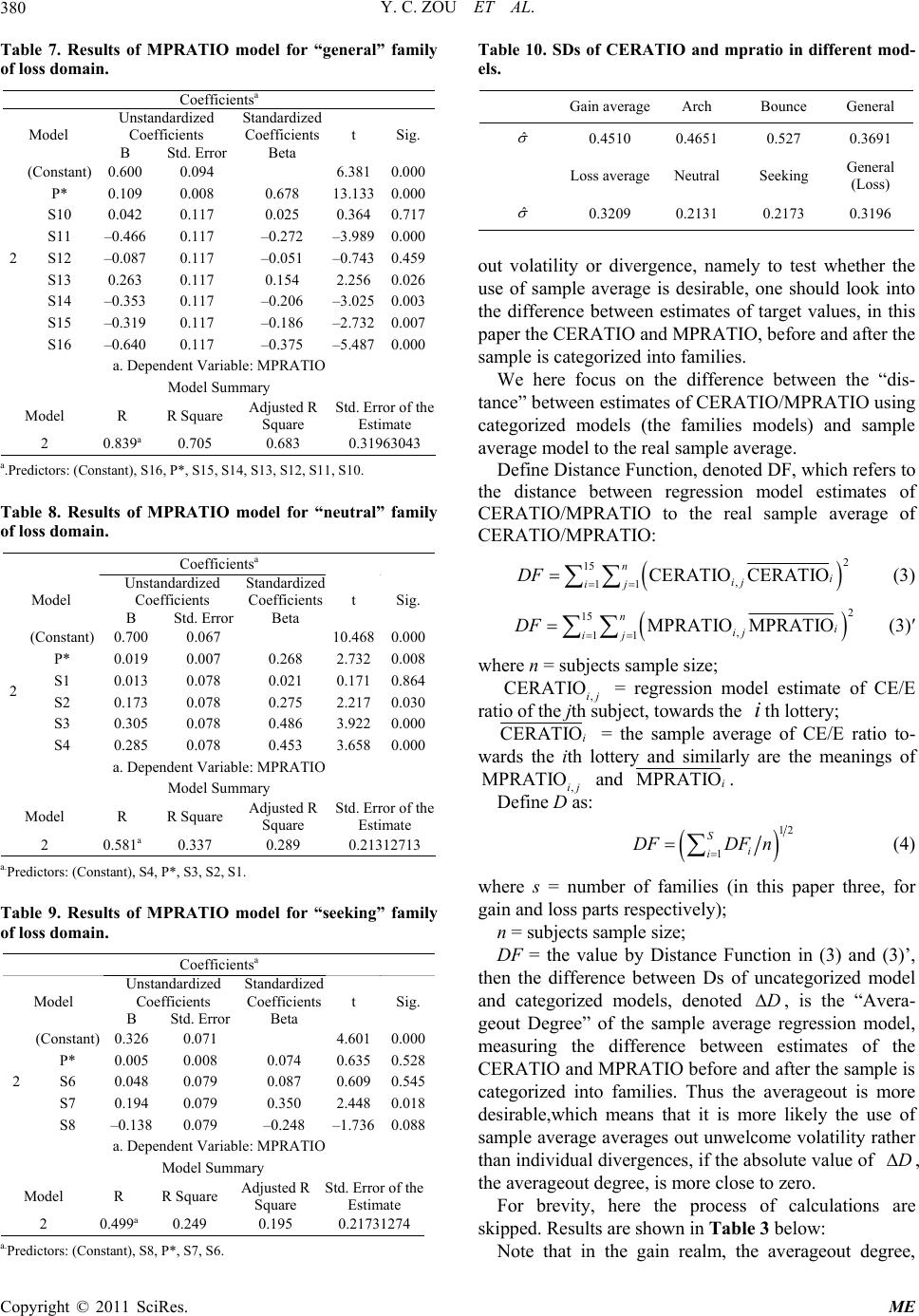

Y. C. ZOU ET AL. 380
Table 7. Results of MPRATIO model for “general” family
of loss domain.
Coefficientsa
Unstandardized
Coefficients
Standardized
Coefficients Model
B Std. ErrorBeta
t Sig.
(Constant) 0.600 0.094 6.381 0.000
P* 0.109 0.008 0.678 13.1330.000
S10 0.042 0.117 0.025 0.3640.717
S11 –0.466 0.117 –0.272 –3.9890.000
S12 –0.087 0.117 –0.051 –0.7430.459
S13 0.263 0.117 0.154 2.2560.026
S14 –0.353 0.117 –0.206 –3.0250.003
S15 –0.319 0.117 –0.186 –2.7320.007
2
S16 –0.640 0.117 –0.375 –5.4870.000
a. Dependent Variable: MPRATIO
Model Summary
Model R R Square Adjusted R
Square
Std. Error of the
Estimate
2 0.839a 0.705 0.683 0.31963043
a.Predictors: (Constant), S16, P*, S15, S14, S13, S12, S11, S10.
Table 8. Results of MPRATIO model for “neutral” family
of loss domain.
Coefficientsa
Unstandardized
Coefficients
Standardized
Coefficients
Model
B Std. ErrorBeta
t Sig.
(Constant) 0.700 0.067 10.468 0.000
P* 0.019 0.007 0.268 2.7320.008
S1 0.013 0.078 0.021 0.1710.864
S2 0.173 0.078 0.275 2.2170.030
S3 0.305 0.078 0.486 3.9220.000
2
S4 0.285 0.078 0.453 3.6580.000
a. Dependent Variable: MPRATIO
Model Summary
Model R R Square Adjusted R
Square
Std. Error of the
Estimate
2 0.581a 0.337 0.289 0.21312713
a.Predictors: (Constant), S4, P*, S3, S2, S1.
Table 9. Results of MPRATIO model for “seeking” family
of loss domain.
Coefficientsa
Unstandardized
Coefficients
Standardized
Coefficients Model
B Std. ErrorBeta
t Sig.
(Constant) 0.326 0.071 4.601 0.000
P* 0.005 0.008 0.074 0.6350.528
S6 0.048 0.079 0.087 0.6090.545
S7 0.194 0.079 0.350 2.4480.018
2
S8 –0.138 0.079 –0.248 –1.7360.088
a. Dependent Variable: MPRATIO
Model Summary
Model R R Square Adjusted R
Square
Std. Error of the
Estimate
2 0.499a 0.249 0.195 0.21731274
a.Predictors: (Constant), S8, P*, S7, S6.
Table 10. SDs of CERATIO and mpratio in different mod-
els.
Gain averageArch Bounce General
ˆ

0.4510 0.4651 0.527 0.3691
Loss averageNeutral Seeking
General
(Loss)
ˆ

0.3209 0.2131 0.2173 0.3196
out volatility or divergence, namely to test whether the
use of sample average is desirable, one should look into
the difference between estimates of target values, in this
paper the CERATIO and MPRATIO, before and after the
sample is categorized into families.
We here focus on the difference between the “dis-
tance” between estimates of CERATIO/MPRATIO using
categorized models (the families models) and sample
average model to the real sample average.
Define Distance Function, denoted DF, which refers to
the distance between regression model estimates of
CERATIO/MPRATIO to the real sample average of
CERATIO/MPRATIO:


2
15
,
11
CERATIO CERATIO
ni
ij
ij
DF   (3)


15
,
11
MPRATIO MPRATIO
ni
ij
ij
DF   2 (3)′
where n = subjects sample size;
, = regression model estimate of CE/E
ratio of the jth subject, towards the th lottery;
CERATIOij i
CERATIO
MPRATIOij
i = the sample average of CE/E ratio to-
wards the ith lottery and similarly are the meanings of
and
,MPRATIOi.
Define D as:


12
1
S
i
i
DFDF n

 (4)
where s = number of families (in this paper three, for
gain and loss parts respectively);
n = subjects sample size;
DF = the value by Distance Function in (3) and (3)’,
then the difference between Ds of uncategorized model
and categorized models, denoted , is the “Avera-
geout Degree” of the sample average regression model,
measuring the difference between estimates of the
CERATIO and MPRATIO before and after the sample is
categorized into families. Thus the averageout is more
desirable,which means that it is more likely the use of
sample average averages out unwelcome volatility rather
than individual divergences, if the absolute value of
D
D

,
the averageout degree, is more close to zero.
For brevity, here the process of calculations are
skipped. Results are shown in Table 3 below:
Note that in the gain realm, the averageout degree,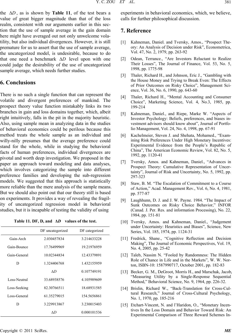

Y. C. ZOU ET AL.381
the , as is shown by Table 11, of the test bears a
value of great bigger magnitude than that of the loss
realm, consistent with our arguments earlier in this sec-
tion that the use of sample average in the gain domain
here might have averaged out not only unwelcome vola-
tility, but also individual divergences. However, it is still
premature for us to assert that the use of sample average,
the uncategorized model, is undesirable, because to do
that one need a benchmark
D
D

level upon with one
could judge the desirability of the use of uncategorized
sample average, which needs further studies.
6. Conclusions
There is no such a single function that can represent the
volatile and divergent preferences of mankind. The
prospect theory value function mistakably links its two
branches in gain and loss domains together, which, albeit
right intuitively, falls in the pit in the majority heuristic.
Also, using sample mean in analyzing data in the studies
of behavioral economics could be perilous because this
method treats the whole sample as an individual and
willy-nilly presumes that the average preference could
stand for the whole, while in studying the behavioral
facts of human preferences, individual divergences are
pivotal and worth deep investigation. We proposed in the
paper an approach toward modeling and data analyses,
which involves categorizing the sample into different
preference families and developing the sub-regression
models. We suggested that this approach is statistically
more reliable than the mere analysis of the sample means.
But we should also point out that our theory still is based
on experiments. It provides a way of revealing the fragil-
ity of uncategorized regression model in behavioral
studies, but it is incapable of testing the validity of using
Table 11. DF, D, and Δ
D
values of the test.
DF uncategorized DF categorized
Gain-Arch 2.030457834 3.214633228
Gain-Bounce 17.76499969 19.21976959
Gain-General 10.02344834 12.43379891
D 1.324406768 1.432155959
D
 0.107749191
Loss-Neutral 33.68938576 4.105989609
Loss-Seeking 82.30766511 18.68931585
Loss-General 61.35279015 154.5656861
D 3.229913867 3.230015403
D 0.000101536
experiments in behavioral economics, which, we believe,
calls for further philosophical discussion.
7. Reference
[1] Kahneman, Daniel. and Tversky, Amos., “Prospect The-
ory: An Analysis of Decision under Risk”, Econometrica,
Vol. 47, No. 2, 1979, pp. 263-92
[2] Odean, Terrance., “Are Investors Reluctant to Realize
Their Losses”, The Journal of Finance, Vol. 53, No. 5,
1998, pp. 1775-98
[3] Thaler, Richard H., and Johnson, Eric J., “Gambling with
the House Money and Trying to Break Even: The Effects
of Prior Outcomes on Risky Choice”, Management Sci-
ence, Vol. 36, No. 6, 1990, pp. 643-60
[4] Thaler, Richard H., “Mental Accounting and Consumer
Choice”, Marketing Science, Vol. 4, No.3, 1985, pp.
199-214
[5] Kahneman, Daniel., and Riepe, Marke W. “Aspects of
Investor Psychology: Beliefs, preferences, and biases in-
vestment advisors should know about”, Journal of Portfo-
lio Management, Vol. 24, No. 4, 1998, pp. 67-91
[6] Kachelmeier, Steven J. and Shehata, Mohamed., “Exam-
ining Risk Preferences Under High Monetary Incentives:
Experimental Evidence from the People’s Republic of
China”, The American Economic Review, Vol. 82, No. 5,
1992, pp. 1120-41
[7] Tversky, Amos. and Kahneman, Daniel., “Advances in
Prospect Theory: Cumulative Representation of Uncer-
tainty”, Journal of Risk and Uncertainty, No. 5, 1992, pp.
297-323
[8] Staw, B. M. “The Escalation of Commitment to a Course
of Action,” Acad. Management Rev., Vol. 6, No. 4, 1981,
pp. 577-87
[9] Laughhunn, D. J. and J. W. Payne. 1984. “The Impact of
Sunk Outcomes on Risky Choice Behavior,” INFOR
(Canad. J. Per. Res. and information Processing), No. 22,
1984, pp. 151-81
[10] Tversky, Amos. and Kahneman, Daniel., “Judgement
under Uncertainty: Heuristics and Biases”, Science, New
Series, Vol. 185, 1974, pp. 1124-31
[11] Fredrick, Shane., “Cognitive Reflection and Decision
Making”, The Journal of Economic Perspectives, Vol. 19,
No. 4, 2005, pp. 25-42
[12] Taleb, Nassim N. “Fooled by Randomness: The Hidden
Role of Chance in Life and in the Markets”, W. W. Nor-
ton, ISBN-10: 1587990717, October 2001, pp. 182-83
[13] Becker, G. M., DeGroot, Morris H., and Marschak, Jacob,
“Measuring Utility by a Single-Response Sequential
Method,” Behavioral Science, No. 9, 1964, pp. 226-32.
[14] Brislin, Richard W., “Back-Translation for Cross-Cul-
tural Research,” Journal of Cross-Cultural Psychology,
No. 1, 1970, pp. 185-216
[15] Etchart-Vincent, N. and l’Haridon, O., “Monetary Incen-
tives In the Loss Domain and Behavior Toward Risk: An
Experimental Comparison of Three Reward Schemes In-

Y. C. ZOU ET AL. 382
cluding Real Losses”, Journal of Risk and Uncertainty, No. 42, 2011, pp. 61-83
Appendix: Replication Experiment of Pros-
pect Theory Problems
PROB1: In addition to whatever you own, you have been
given 1,000. You are now asked to choose between
A: 50% chance to win 1,000 B: a sure gain of 500
PROB2: In addition to whatever you own, you have
been given 2,000. You are now asked to choose between
A: 50% chance to lose 1,000 B: a sure loss of 500
PROB3: Choose between:
A: 25% to win 6,000
B: 25% to win 2,000 and another 25% to win 4,000
PROB4: Choose between:
A: 25% to lose 6,000
B: 25% to win 2,000 and another 25% to lose 4,000