 Materials Sciences and Applications, 2015, 6, 978-994 Published Online November 2015 in SciRes. http://www.scirp.org/journal/msa http://dx.doi.org/10.4236/msa.2015.611098 How to cite this paper: Billaud, G., El Ouafi, A. and Barka, N. (2015) ANN Based Model for Estimation of Transformation Hardening of AISI 4340 Steel Plate Heat-Treated by Laser. Materials Sciences and Applications, 6, 978-994. http://dx.doi.org/10.4236/msa.2015.611098 ANN Based Model for Estimation of Transformation Hardening of AISI 4340 Steel Plate Heat-Treated by Laser Guillaume Billaud, Abderazzak El Ouafi, Noureddine Barka Mathematics, Computer Science and Engineering Department, University of Quebec at Rimouski, Rimouski, Canada Received 7 October 2015; accepted 15 November 2015; published 18 November 2015 Copyright © 2015 by authors and Scientific Research Publishing Inc. This work is licensed under the Creative Commons Attribution International License (CC BY). http://creativecommons.org/licenses/by/4.0/ Abstract Quality assessment and prediction becomes one of the most critical requirements for improving reliability, efficiency and safety of laser surface transformation hardening process (LSTHP). Accu- rate and efficient model to perform non-destructive quality estimation is an essential part of the assessment. This paper presents a structured and comprehensive approach developed to design an effective artificial neural network (ANN) based model for quality estimation and prediction in LSTHP using a commercial 3 kW Nd:Yag laser. The proposed approach examines laser hardening parameters and conditions known to have an influence on performance characteristics of hard- ened surface such as hardened bead width (HBW) and hardened depth (HD) and builds a quality prediction model step by step. The modeling procedure begins by examining, through a structured experimental investigations and exhaustive 3D finite element method simulation efforts, the rela- tionships between laser hardening parameters and characteristics of hardened surface and their sensitivity to the process conditions. Using these results and various statistical tools, different quality prediction models are developed and evaluated. The results demonstrate that the ANN based assessment and prediction proposed approach can effectively lead to a consistent model able to accurately and reliably provide an appropriate prediction of hardened surface character- istics under variable hardening parameters and conditions. Keywords Laser Hardening Process, AISI 4340 Steel, Case Depth, Hardened Bead Width, Artificial Neural Netwo rk  G. Billaud et al. 1. Introduction In the industry, many steel components require a surface heat treatment in order to have the desired surface qualities such as hardness and wear resistance. Among the available processes, laser hardening process (LHP) is one of the most efficient, as it allows a very fast and localized metallurgical transformation. In addition, the process generates a hard surface layer with low distortion [1]. Using high energy beam, the surface is rapidly heated to reach the transition temperatures (microstructure changes) before being quenched by heat conduction into the colder core of the material. Consequently, a martensitic layer is produced without affecting the core of the material [2]. Despite its industrial advantages, pred icting hardness profiles with a good accuracy remains difficult. Indeed, besides the process parameters (Power, scanning velocity and focus diameter), which can be properly set, the process is affected by the non-line ar b ehavio r o f the r mo -physical and metallurgical properties of the material [1]. It makes the temperature distribution uneasy to predict by complicating the resolution of the governing heat- flow equation. Experimental tests are also expensive in terms of time and resources, especially if one wants to test many combinations of control parameters to have a better understanding of the process. Among all the approaches that can be used to understand the process and ultimately to predict its performance, 3D simulation represents a powerful tool for combining multi-physics problems and taking into account the ma- terial and complex geometries. In fact, the developed model includes the non-linear properties of the material and the heat-flow equation is solved using the finite element method (FEM) [3] [4]. The FEM enables solving the governing heat-flow equation that determines the temperature distribution for each time step during the heating process. The hard ness is t hen appr oximated by the equations of Ashby and Eas t erling [5]. The advant age of the simulation is that, although it might be long and tedious to implement, once it is completed and experi- mentally verified in a few cases, one can test any combination of input parameters and quickly generate a large number of data which can be used for further exploitation. Many studies have been conducted to optimize the various laser process parameters (surface hardening, laser welding, laser cutting, etc.) through statistical meth- ods such as the ANOVA method. It can be applied in many fields of engineering, including production proc- esses and products for professional and consumer markets all over the world [6]. S-L Chen a nd D. She n [7] used the Taguchi tools such as graphic designs of parameters and analysis of variance (ANOVA) to optimize the hardened depth (HD) and the hardened bead width (HBW) in the case of the LHP. Bad kar and Pandey [8] used the same tools to determine the relative importance of each parameter on the LHP. K.Y. Bentounis, A.G. Olabi and M.S.J. Hashmi [9] conducted a similar study in the case of a laser welding process. Most recently, Sathiya et al. [10] also used the Taguchi method to optimize the laser welding parameters. Given that experimental char- acterization requires great efforts in terms of time and money, it is not easy to experiment all the combinations of the input parameters. The Taguchi method reall y is an asset, as it is a partial factorial design that only requir es some combinations of the input parameters in order to be performed and yet, it gives accurate statistical results in the overall process. Others studies are conducted using artificial neural networks (ANN) in order to improve the performance of the laser processes [11]. Ciurana J. et al. [12] used ANNs to establish a model for laser micromachining of hardened steel and to optimize the process parameters. Pan Q.Y et al. [13] performed a similar study by using a neural network to model the non-linear relationship between laser processing parameters and corrosion resis- tance of the surface of stainless steel during the process of laser surface re-melting, which loc ally improved the corrosion resistance of the steel. Munteanu and Adriana [14] predicted the surface hardness of steel usi ng a ne u- ral network in the case of an electron beam machining process which is similar to the LHP. F. Lambiase et al. developed a prediction model of laser hardening by means of an ANN using experimental datasets and linear interpolatio ns between those experimental measures to train the network. Ho wever, to obtain good and efficient modeling results with ANN techniques, a large quantity of experimental data is advantageous and the observa- tions should cover a sampling space as wide as possible in order to simplify the interpolation task. Indeed, in any modelling experi ment, the results depend, to a large degree, on the method used to collect data. In a lot of cases, full factorial experiments are conducted. This appro ach cannot be implemented when too many factors are under consideration, because the number of repetitions required would be prohibitive in time and cost. Regular fractional factorial designs cannot produce credible results when interactions among the factors exist. By contrast, the use o f a testing strategy such as the orthogonal arrays (OAs) developed by Taguchi leads to an efficient and ro bust fractional factorial desig n of experiments that can collec t all the statistically significant da ta 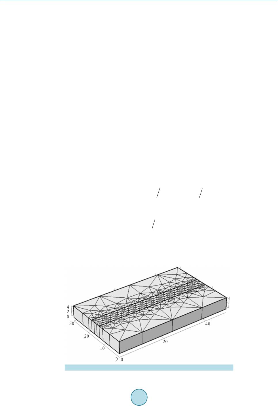 G. Billaud et al. with a minimum number of repetitions. Accordingl y, OAs a re use d in th is st ud y fo r t he exp e ri ment al d e s ig n. On the ot her hand, by using 3D FEM simulation tha t can provide results matching fairly well with the experimen- tally observed variables, one can easily and quickly obtain additional data for any combination of input parame- ters. The quantity of simulated data generated in a short time compared to experimental data would allow ex- haustive statistical analysis including all levels of all input parameters. Moreover, with a large quantity of data for training, a simple Multilayer Perceptron ANN can be appropriate for modeling. The objective of this paper is to present a str uctured a nd compre hensive a ppro ach develop ed to de sign an ef- fective artificial neural network (ANN) based model for quality estimation and prediction in LSTHP using a commercial laser source. The proposed approach examines laser hardening parameters and conditions known to have an influence on performance characteristics of hardened surface such as hardened bead width (HBW) and hardened depth (HD) and builds a quality prediction model step by step. The modeling procedure begins by examining, through a structured experimental investigations and exhaustive 3D FEM simulation efforts, the relationships between laser hardening parameters and characteristics of hardened surface and their sensitivity to the process conditions. Using these results and various statistical tools, different quality prediction models are developed and evaluated. In order to carry out the models building procedure, an efficient modeling plan- ning metho d c o mbini ng ne ur a l networks p ar a di gm, a multi-criter ia optimization and various statistical to ols is adopted. 2. 3D Model Implementation and Validation 2.1. Implementation The 3D FEM model is developed on the commercial software to estimate the temperature profiles. These tem- perature profiles are used to approximate the surface hardness profiles (surface hardness, HD, HBW ) . T he part is a 50 mm × 30 mm × 5 mm parallelepiped (Figure 1). In this stud y, the heat f lux used for the si mulation is con side re d as a Ga ussian bea m distribution type which is given by Equation (1) [1], ( ) ( ) [ ] ( ) () { } 22 22 00 0 exp2 2E ExxVtwyyw =×−−+×+ − (1) where V is t he sc an ning velo cit y, and x0 and y0 are the beam center coordinates at t = 0 s. E (W/m2) represents a Gaussia n heat flux moving according to the x-axis at the velocity V. E0 is defined by Equation (2), (2) where w i s the Gaussia n beam ra dius, P is the laser beam power, Rc is the reflectio n coefficient of the mater ial surface [2]. The movin g isot her mal cont our s can b e o bse rved in Figure 2. B ecause of the Gaussian form of the beam, the temperature is at its maximum (about 1110 K) at the center of the spot. The temperature decreases rapidly with Figure 1 . Sample with its mesh implemented on COMSOL. 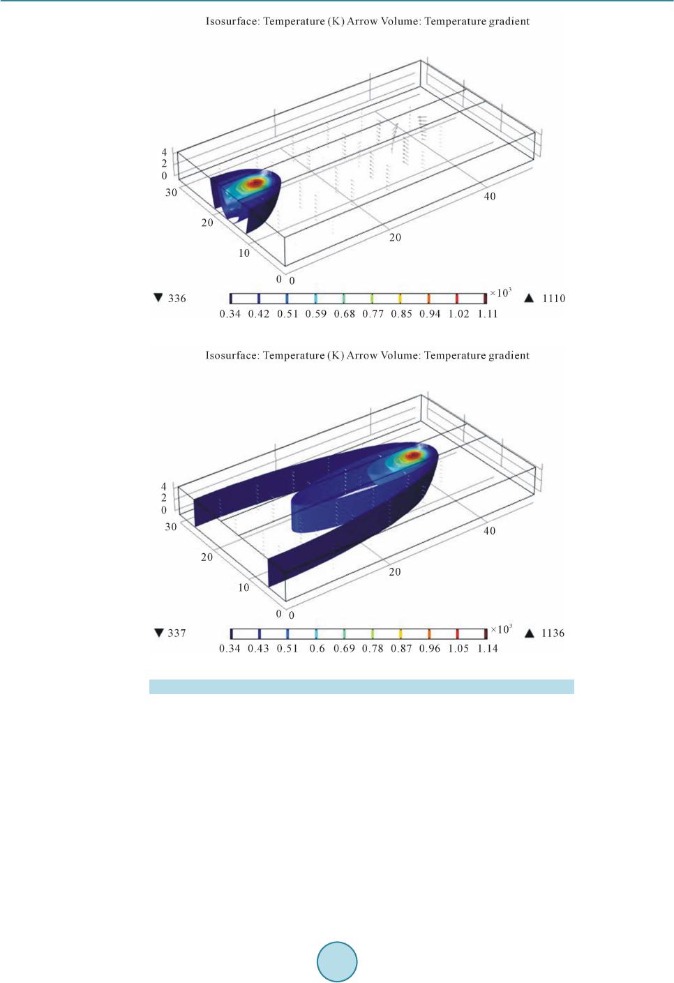 G. Billaud et al. (a) (b) Figure 2 . Isothermal contours: (a) t = 0.4 s and (b) t = 2.5 s. the depth because of heat conduction into the colder core of the material. The heated volume is small at the be- ginning of the process (t = 0.4 s) and it gets larger as the time passes and the bea m moves (t = 2.5 s). As it can be seen i n Figure 2, the small volume of the part that had reached the temperature of 1110 K at t = 0.4 s (see Fig- ure 2(a)) cool downed to reach a temperature under 430 K at t = 2.5 s (see Figure 2(b)). It means that a very fast quenching hap pened in t hat volume. Once the temperature distribution is determined, the hardness profile is estimated using the equations of Ashby and Easterling [5]. Those equations are implemented in MATLAB® to obtain the hardness at any point belonging to the heated part and, conseque ntly, the hardness curve rep resent ing t he hardness versu s dep t h. The 4340 steel properties are displayed in Table 1. The specific heat and the thermal conductivity are temperature dependant and their dependency is taken into account in our model .  G. Billaud et al. Table 1. Metallurgical properties. Property Symbol Unit Value Reflecti o n coefficient Rc 0.6 Eutectoi d temperature Ac 1 K 996 Austenitization temperature Ac3 K 1053 Austeni te gra i n size (assumed) g µm 10 Activation energy of carbon diffusion in ferrite Q kJ/mol 80 Pre-exponent ial for dif fusion of carbon D0 m2/s 6 × 10⁻⁵ Gas constant R J/mol·K 8.314 Steel carbon conten t C 0.43% Austenite carbon content Ce 0.8% Ferrite carbon content Cf 0.01% Critical value of carbon content Cc 0.05% Volume fraction of pearlite colonies fi 0.5375 2.2. Metallurgical Equations When the temperature in the material reaches the eutectoid temperature Ac1 in a small volume under the surface, the steel microstructure, which is generally tempered martensite in the case of the steel AISI 4340, starts to transform into austenite. The complete transformation from tempered martensite to austenite occurs when the temperature reaches Ac3. In the case of laser hardening treatment, when the temperature drastically decreases due to rapid heat diffusion into the colder core of the part, the austenite transforms into hard martensite. This is what is called a heat cycle (Figure 3). As see n on Figure 3, the peak temperature at the surface is above Ac3. Therefore, a complete transformation into hard martensite happened at the surface. However, the peak temperature at 1.4 mm under the surface is un- der Ac1. It means that no transformation happened a t this dep th. The to ta l nu mber o f d iffus i ve j u mps t hat o c cur d uri n g the heat c ycl e a f fect s the e xtent o f the str uctura l c ha nge and is given b y the kinetic strength I [1] [5], [ ] ( ) { } exp dIQR Ttt= −× ∫ (3) where Q is the activation energy for the transformation and R is the gas constant. It is more convenient to ex- press I as described in Equation (4). (4) Here Tp is the peak te mperature at the co nsidered depth and τ is the thermal time constant. The terms α and τ are approximated by Equations (5) and (6), (5) ( ) ( ) 10 12π p RcPKe VTT τ =−− (6) where T0 is the initial temperature. The obtained austenite has the same carbon content as a perlite microstructure Ce = 0.8%. From there, the carbon diffuses into the proeutectoid ferrite. When the temperature reaches Ac1, the volu me fraction of a ustenite is fi ( which is also the minimum volume fraction of martensite), gi ven by Equa tio n (7), () () 0.8 0.8 if f f CCCC=− −≈ (7) where Cf is the negligible carbon content of the ferrite and C is the carbon content of the steel. 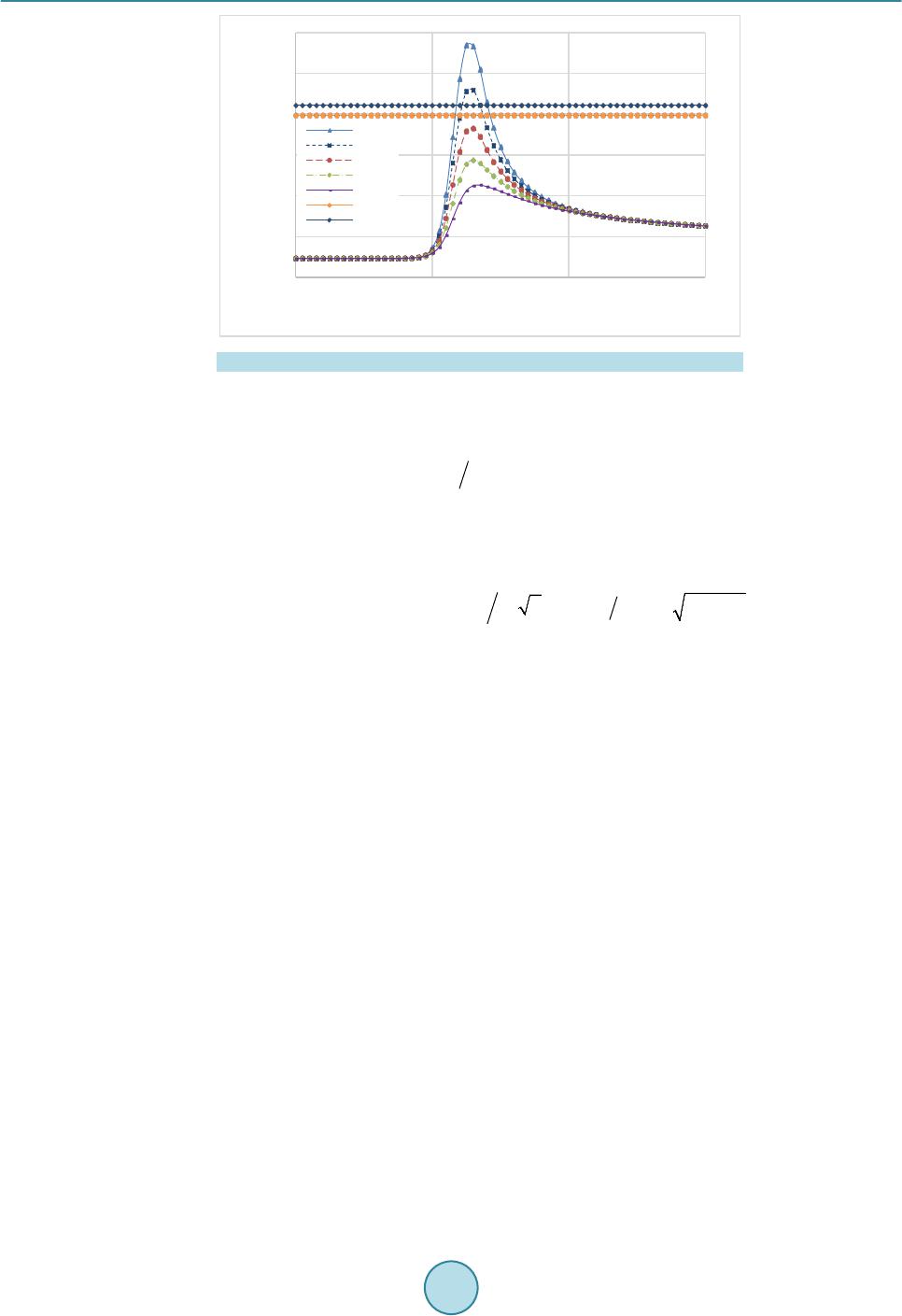 G. Billaud et al. Figure 3 . Temperature evolution at different depths (850 W and 9 mm/s). The maxi mum martensite fraction allowed by the trans formation te mperature time diagram (TTT diagram) is () ( ) ( ) 1 1 3113 1 0 if 1 if 0 if p ip p p fmT Ac fmfif TAcAcAcAcTAc fmT Ac = < = +−−−<< = < (8) Ashby and Easter ling supposed that all the material with a specific ca rbon propor tion above the critical value Cc will transfor m into martensite. The volume fraction of the martensite is then given by Equation (9 ) [1] [5]. ( ) ( ) ( ) () () { } 2/3 0 exp 12πln 2 i iec ffmfm ffgCCDI = −−×−×× (9) Here g is the mean grain size and D0 is the diffu sio n constant for the car bon in ferrite. The hardness can then be calculated by a mixture rule (Equation (10)). (10) The value Hm and Hf+p are given by Maynier equations that take in account the cooling rate and the composi- tion of the material [15]. 2.3. Experimental Validation The experimental procedure consists of a first heat treatment in a furnace with a water quenching followed by a tempering at 640˚C for 1 hour . T he ai m is to r each a homogene ous hardness of 440 HV for all t he samples. Then, a commercial 3 kW Nd:Yag laser power (IPG YLS-3000-ST2), combined with a 6 degrees of freedom articu- lated robot (Figure 4) is used to perform laser heating. The plan-parallel sample is put on a metal plate under the laser head. This type of laser generates a laser beam with a wavelength λ = 1064 µm. The p r o cess parameters are the input power, the scanning velocity and the focus diameter. In this study, the laser beam has a straight-line trajectory as seen in Figure 2. Finally, the resulting case d e pth is measured by micro indentation. Experimental validations are conducted according the Table 2. The focus diameter is 1260 µm for the three tests. The values are chosen so that the surface temperature reaches the austenite temperature Ac3 but does not hit the melting temperature (about 145 0˚C). A mic r o -hardness machine is used to characterize the hardness curve as a function of the depth. After the laser treatment, the samples are prepared and polished to reach adequate surface finish. The hardness is then meas- ured by using a micro -hardness machi ne. The validation i s conducted by micro indentation, with 100 µm steps between consecutive Vickers marks on the surface along a vertical axis. The experimental results help to vali- date and calibrate the model. In this sense, the obtained results confirm the concordance between the experi- mental and simulated hardness curves. This suggests that even if the developed model is not able to accurately 200 400 600 800 1000 1200 1400 0123  G. Billaud et al. Figure 4 . Experimental setup for model validation. Table 2. Experimental matrix for validation. Test Powe r (W) Scanning velocity (mm/s) 1 850 9 2 850 12 3 950 12 predict the hardness curve, it can determine the hardened depth with good accuracy. Figures 5-7 show a com- parison between the simulated and measured hardness curve using Vickers hardness scale (VH) for the three tests (Table 2). It is worth noting that the developed 3D model is unable to predict the over-tempered zone where the hardness of the material becomes inferior to the initial hardness. However, hardened zone, transition zone and unaffected zone are correctly predicted. As expected, the hardened depth (at the start of the transition zone) increases as the power rises and/or the scanning velocity decreases. Table 3 shows the average absolute and relative errors between measured and simulated hardness. The preliminary tests allow to conclude that, de- spite the difference of more than 50 HV in terms of absolute error, the relative error is very small, not exceeding 10%. As sho wn in Figures 5-7, the si mulation is fairly accurate in both hardness prediction and case depth pre- diction. 3. Calibration of the Model with Corrected Rc The coefficient Rc can be estimated around 0.6 for steel [2]. However, this coefficient greatly varies according to the surface temperature. Moreover, the surface temperature depends on the process parameters. In order to correctly calibrate Rc, different combinations of process parameters are executed using laser heating cell and the Rc is corrected so the results generated by the simulation match the experimental results for each set of input parameters. Finally, Rc is approximated as a function of the process parameters using a linear regression tech- nique. Tab le 4 shows the Rc values depending on the laser p ower, the scanning velocity and the focus radius of the beam spot. The coefficient seems to increase as the power and/or the scanning velocity increases. Also, it seems to decrease when the focus radius increases. The regression equation (Equation (11)) proves that there is a linear relationship between Rc and the process parameters. The correlation coefficient is 0.994, which confirms a good correlation. Rc0.42050.000303 P0.003553 V0.000198Rad=+×+×−× (11) P is t he inp ut po wer i n W, V is the sca nni ng velo city i n mm/ s, and Ra d is t he foc us radi us in µ m. The d evel- oped equation is incorporated in the simulation model. The HD and HBW can be estimated with good accuracy as a function of the process parameters. 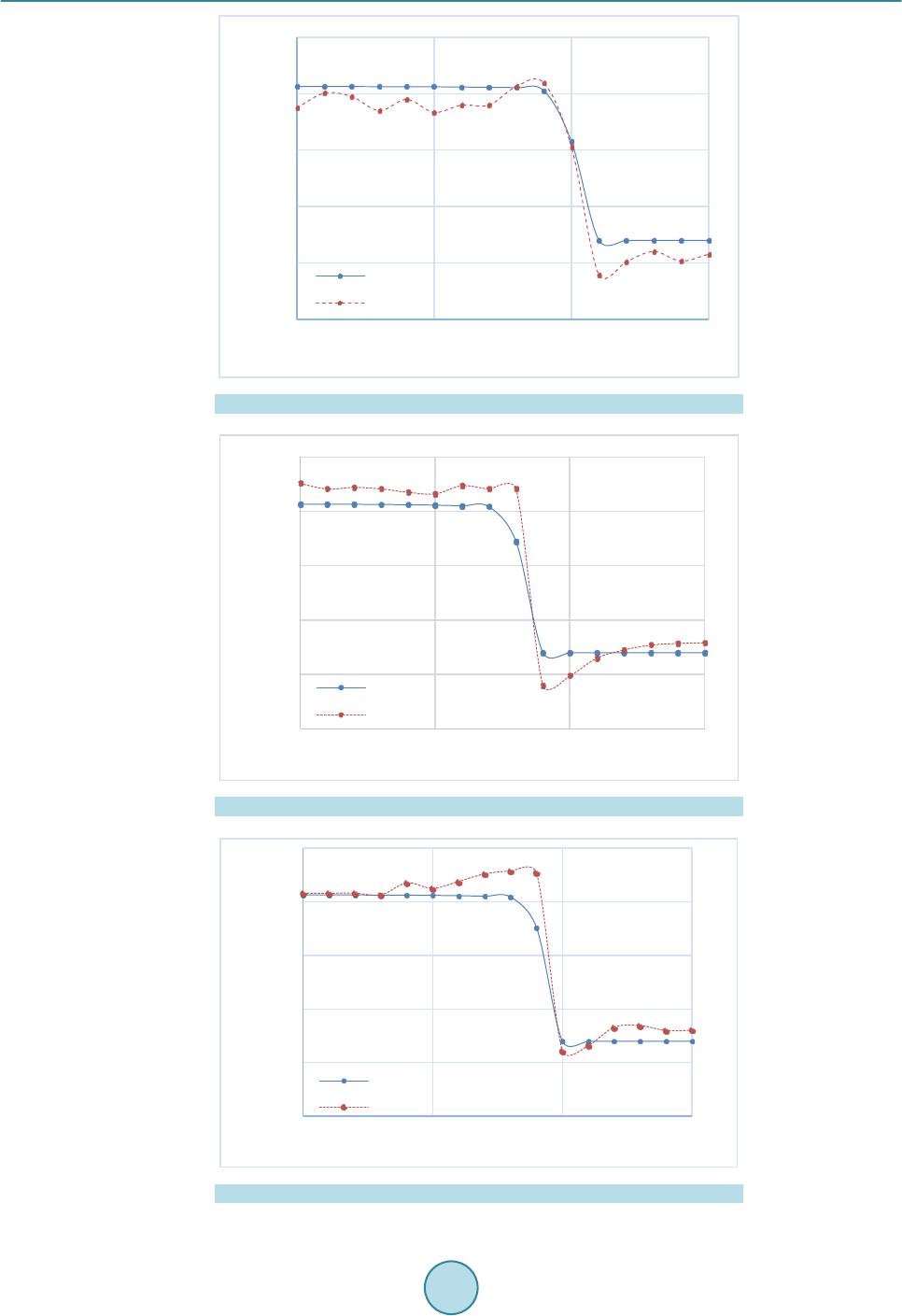 G. Billaud et al. Figure 5 . Hardness curve for test 1 (850 W and 9 mm/s). Figure 6 . Hardness curve for test 2 (850 W and 12 mm/s). Figure 7 . Hardness curve for test 3 (950 W and 12 mm/s). 300 400 500 600 700 800 05001000 1500 Simul ated ha rdnes s (HV) Meas ured hardne ss ( HV) 300 400 500 600 700 800 05001000 1500 Simul ated ha rdnes s (HV) Meas ured hardne ss ( HV) 300 400 500 600 700 800 05001000 1500 Simul ated ha rdnes s (HV) Meas ure d har nes s ( HV )  G. Billaud et al. Table 3. Average absolute and relative hardness errors resulting from the preliminary tests. Test Absolute error (HV) Relative error (%) 1 43 8.8 2 30 5.2 3 24 4.0 Table 4. Corrected R c according to process p arameters. Power P (W) Scanning veloci ty V (mm/s) Focus radius Rad (µm) Correc ted Rc 400 20 550 0.50 520 20 550 0.54 630 20 550 0.57 740 20 550 0.61 400 12 550 0.47 400 16 550 0.49 400 16 480 0.51 400 16 613 0.48 400 16 663 0.47 4. Shadowgraph Measurement As this stud y is focused on the HD and HBW and not the hardness values themselves, the depth and width are measured using optical method based on shadowgraph measurement. Figure 8 shows a micrographic picture o f a part heat treated by laser with a power of 1000 W and a scanning velocity of 12 mm/s. The hardened region with hard martensite appears very clearly after a chemical treatment and can even be observed with the naked eye. Two sig ni ficant z o ne s c a n b e d istin g uis hed . T he fir s t one i s the melted re gion near the surface that received a great amount of energy, enough to reach the melting point. The second region represents the hardened region where the temperature exceeded the austenitization temperature (Ac3) without reaching the melting point and where the micro str ucture chan ged into martensite upon self-quenching. 5. Statistical Study In the p re sent study, the objective is to predict the HD and HBW with given process parameters provided by the great number of data generated through simulation (assuming the input parameters are included in the range of study). A statistical study is conducted through a design of experiment (DOE) to determine the relative signifi- cance of each parameter and the interactions between them. The ANOVA method aims to study the effects of parameters on the hardness. It gives the contribution of each parameter on the variation of the outputs (HD and HBW). The process parameters and their design levels are displayed in Table 5. The levels are chosen so that the surface transformation happens and the surface temperature does not hit the melting temperature regardless of the combination of process parameters. The simulatio n allowed us to quickly ob tain result s for all 64 (43) possible combinatio ns of factor level s, and thus to generate a full factorial design. Statistical studies such as analysis of variance, main effects studies and linear regression are conducted. 5.1. ANOVA for HD versus P, V and Rad Table 6 presents the detailed statist ical analysis. An F-value above 11.77 implies that the parameter is very sig- nificant. In this case, power (P), scanning velocity (V), focus radius (Rad) are all significant models terms. The interaction terms are less important since their contributions are less than 0.4%. Also, it is clear that the power 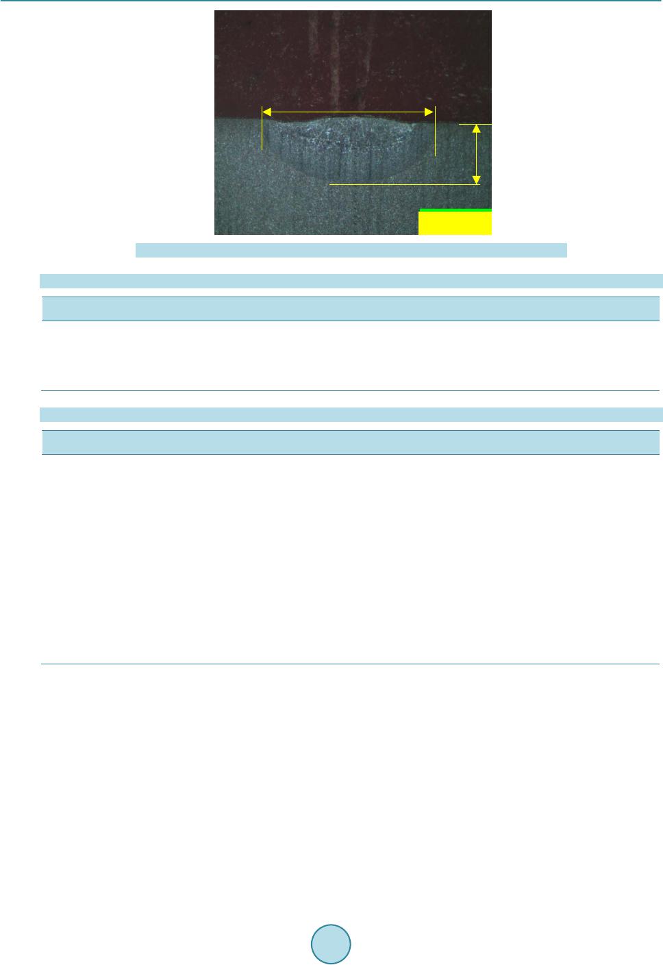 G. Billaud et al. Figure 8 . Micro graphic pictu r e illustrating the HBW and HD after ch emical etchi ng. Table 5. Factors and levels used for the ANOVA study. Fac to rs Factor Levels Laser Power (P) [W] 410 520 613 740 Scannin g Velocit y (V) [mm/s] 12 16 18 20 Focus Radius (Rad) [µm] 480 550 613 663 Table 6. ANOVA for HD. Source DF SS contribution MS F-value p-value P 3 563906 48.4% 1879 69 499.71 0.000 V 3 568906 48.8% 189635 504.14 0.000 Rad 3 13281 1.1% 4427 11.77 0.000 P × V 9 4531 0.4% 503 1.34 0.264 P × Rad 9 2656 0.2% 295 0.78 0.632 V × Rad 9 2656 0.2% 295 0.78 0.632 Model 36 1155936 99.1% 383124 Error 27 10158 0.9% 376 Total 63 1166094 and the scanni ng veloci ty hav e the large st effec t on the res ponse val ue and that they are equival ent wit h contri- butions around 48%. The three interaction terms can be considered negligible. Figure 9 shows the effect of all parameters on the case depth (HD). The obtained results confirm that the HD increases as beam power increases and/or as scanning velocity decreases. It also increases as the focus radius decreases. The ANOVA method is conducted in order to assess the significance of each parameter. For each pa- rameter studied, the variance ratio value, F, is compared to the values from standard F-tables for gi ven stati stical levels of significance. In this way, it is concluded that within the invest igated processing ranges, the power, the scanning velocity and the focus radius are significant for the case depth at 95% confidence. Since the interaction terms have negligible contributio ns, they will not be conside red in the rest o f the study. Figure 10 shows the HD calculated using the regression formula (Equation (12)) for all 64 combinations of process parameters and their distribution around the bisector of the quadrant. If the formula is perfectly accurate, all the points should be on the bisector. For the regression formula to be considered accurate, a maximum relative error of 10% is allowed Har dene d be ad w idth ( HB W ) Hardened depth ( HD) 1 mm 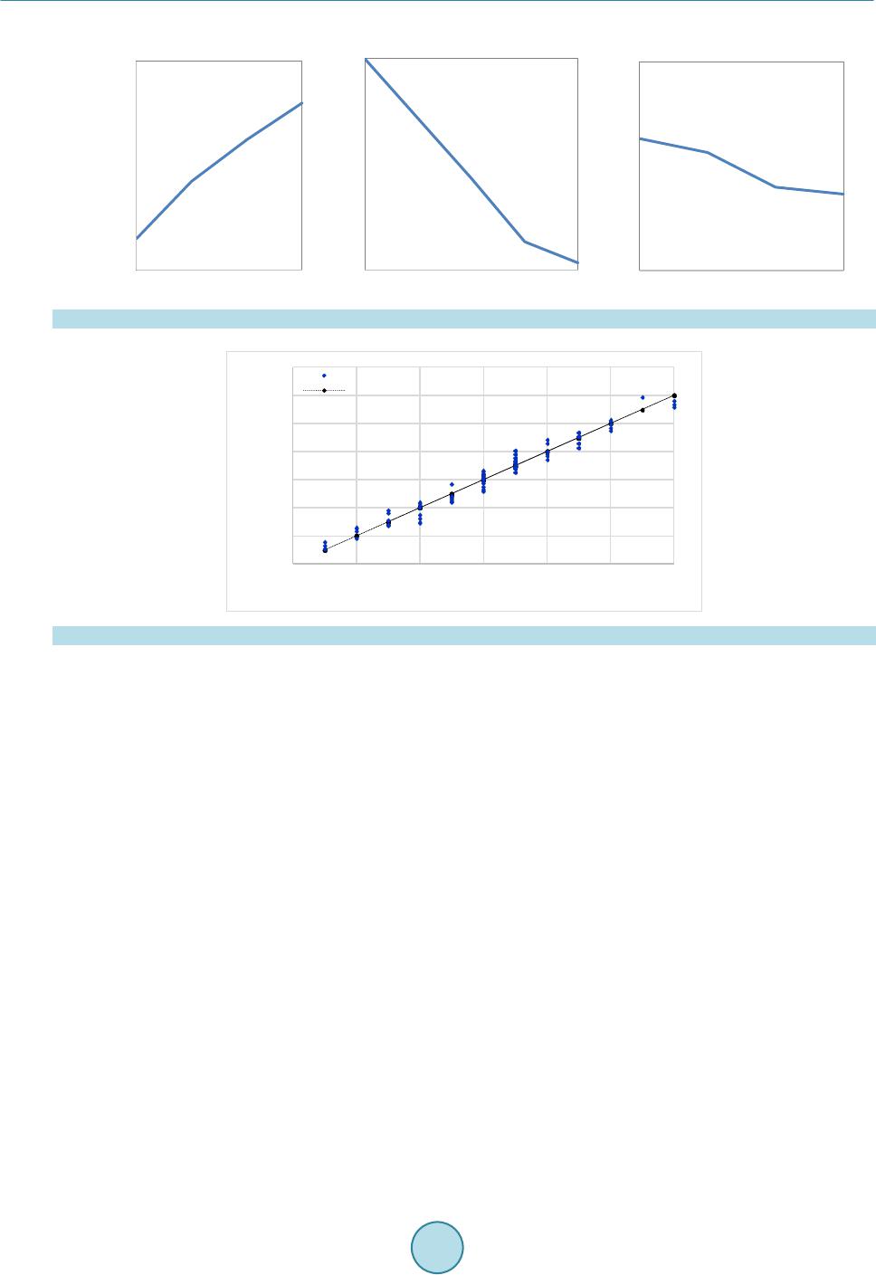 G. Billaud et al. Figure 9 . Effects of parameters o n case depth. Figure 10. Comparison between simulated HD and HD calculated by regression formula (Equation (12)). for all 64 sets of process parameters. A maximum relative error of 6.51% is observed, with a mean relative error of 2.25% between the HD calculated with the regression formula and the one simulated by the software. The coefficient of deter mination R2 is mainly used to measure the relationship between experimental data and meas- ured data. A coefficient R2 = 99.13% indicates an accurate study. HD1113.70.7557P31.70 V0.2036 Rad=+×−× −× (12) 5.2. ANOVA for HBW versus P, V and Rad Table 7 shows the detailed statistical analysis. An F-value above 70.68 implies that the parameter is very sig- nificant. In this case, power (P), scanning velocity (V), focus radius (Rad) are all significant models terms. The interaction terms are less important since their contributions are less than 0.7%. Also, it appears that the input power and the scanning velocity have the largest effect on the response value with contributions around 37% - 43%. The three interaction terms can be considered negligible. The coefficient of determination R2 is mainly used to measure the relationship between experimental data and measured data. Just like for the hardened depth, the input laser power and the scanning velocity have the same degree of impact (and the opposite effect); the other parameter (Rad) still have significance, and the interactions are negligible. The fir st t hin g one c an no ti ce on Fig ure 11 is that the main effects plot for H BW is similar to the main effects plot for the HD, with the noticeable exception of the focus radius, which has the opposite effect on the HBW compared to the effect it has on the HD. Indeed, when the focus radius increases the HBW increases as well, whereas the HD decreases (see Figure 9 and Fig ure 11). This is caused b y the Gaussia n distribution of the en- ergy at the surface of the material, which results in a relationship between HD and HBW. Indeed, the fact that the radius is greater while the power and the scanning velocity remain the same means that there will be less en- ergy at the center of the focus. 700 800 900 1000 1100 410 520 630 740 600 700 800 900 1000 1100 1200 1300 600 700800 900100011001200 Simulated hardened depth (µm) Statistica lly calculate d HD (µm) 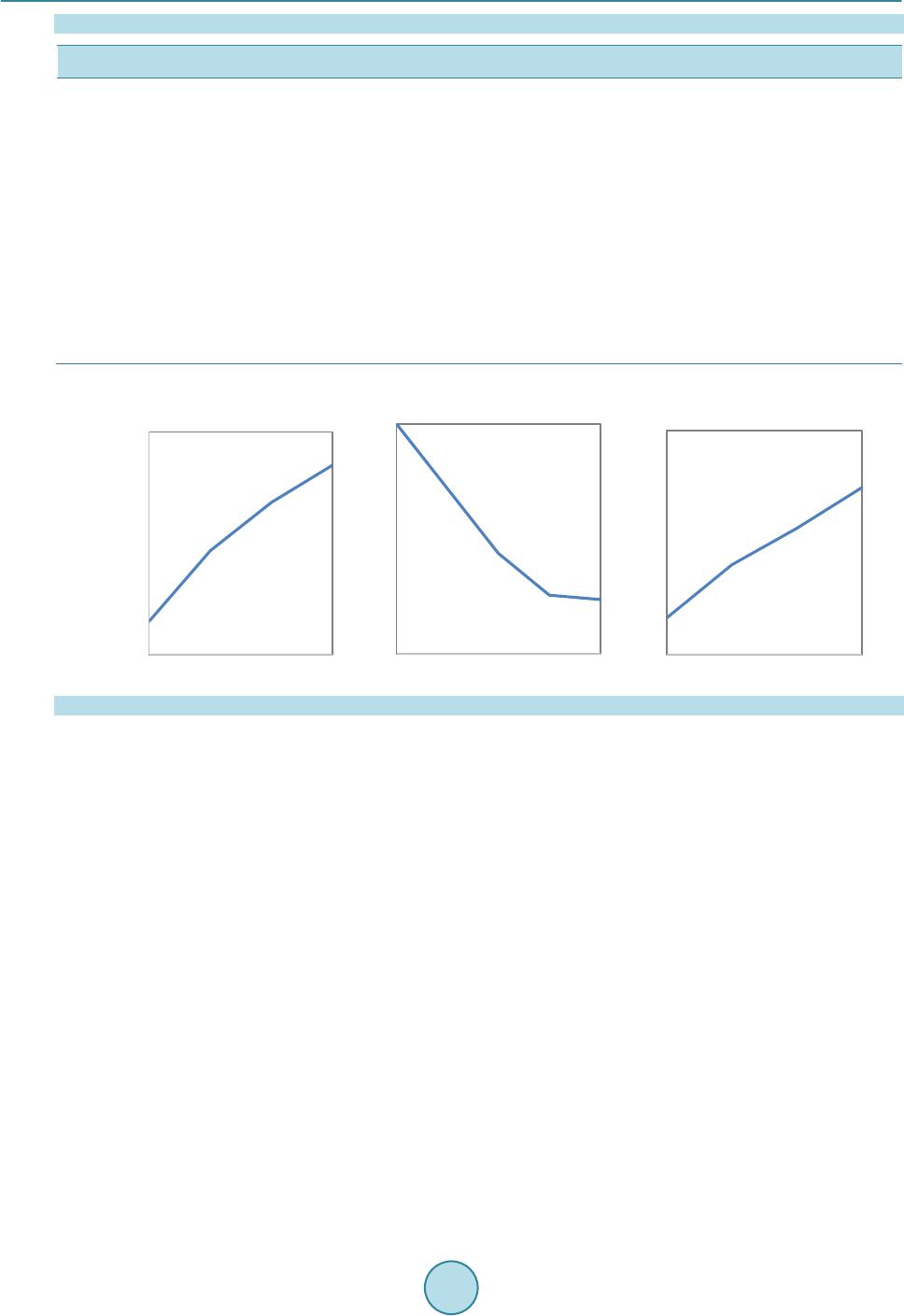 G. Billaud et al. Table 7. Resu l ts of the ANOVA for HBW. Source DF SS Contribution MS F-value p-va lue P 3 1763125 37.4% 587,708 161.71 0.000 V 3 2023125 43% 674,375 185.56 0.000 Rad 3 770625 16.4% 256,875 70.68 0.000 P × V 9 13125 0.3% 1458 0.40 0.923 P × Rad 9 30625 0.7% 3403 0.94 0.511 V × Rad 9 10625 0.2% 1181 0.94 0.959 Mode l 36 4611250 98% 1525,000 Error 27 98125 2% 3634 Total 63 4709375 Figure 11. Main effects plot for hardened bead width. As for the HBW , it appears that the interactions are negligib le with very low F-value. Ther efore they will no t be include d in the re gres s i on e quation. Figure 12 shows the HBW calculated using the regression formula (Equation (13)) for all 64 combinations of process parameters and their distribution around the bisector of the quadrant. If the formula is perfectly accurate, all the points should be on the bisector. A maximum relative error of 6.95% is observed, with a mean relative error of 2.39% between the HBW calculated with the regression for mula and the one simulated by the software. Bo t h value s are well under the maximum criteria of 10% and thus, t he fo rmula can be considered accurate. Moreover, the coefficient of determination R2 = 97.92% testifies an accurate regression equation albeit not as satisfying as it is for the HD. HBW1782 1.3409 P57.68 V1.598 Rad=+×−× +× (13) In addition to the statistical stud y, and in order to provide a reliable alte rnative to standard ther mal techniques that would be accurate and less time consuming, we conducted a study with an artificial neural network (ANN). 6. Neural Network Modeling As compared to other techniques, a n ANN provides a more effective modeling capability, particularly when the relationship between sensor-derived information and the characteristic(s) to be identified is non-linear. ANNs can handle strong non-linearity, a large number of variables, and missing information. Based on their intrinsic learning capabilities, ANNs can be used in a case where there is no exact knowledge concerning the nature of the relationships between various variables. This is very useful in reducing experiment effor ts. 2200 2300 2400 2500 2600 2700 2800 410 520 630 740 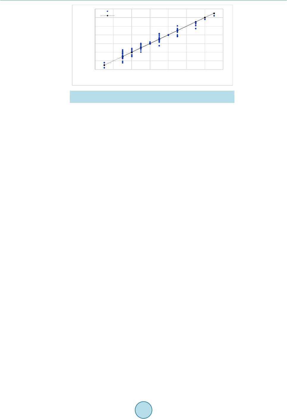 G. Billaud et al. Figure 12. Comparison between simulated HBW and HBW calculated by regression formula (Equation (13)). A neural network is used to predict the hardened depth and hardened bead width. Neural networks are gener- ally presented as systems of interconnected neurons, where the links between neurons are weighted. Figure 13 shows the general principle of an ANN model. The goal is to produce one or more outputs that reflect the user-defined i nformation sto re d in the con nections d uring t ra i ning. In this stud y, a Generalized Feed-Forward M ultilayer Pe rceptro n (GFF-M LP) neura l netwo rk mode l with one hidd en layer co ntainin g 7 neuro ns is chosen. Whil e vario us ANN te chniques can be used in this ap proac h, gen- eralized feed forward networks seem to be the most appropriate because of their simplicity and flexibility. Be- fore selecting the variables and training the models, it is important to establish the network topology and opti- mize the training performances. The idea is to approximate the relationship between the ne t work p ar a me te rs a nd the complexity of the variables to be estimated. The selected network is that which achie ved the bes t res ults, the [n|2n+1|3] network, where n is the number of inputs. The perceptron is characterized by a nonlinear sigmoid function. This type of neural network is always fully connected, meaning each perceptron of each layer is con- nected with all the perceptrons in the previous layer [16]. In a G FF-MLP network, connections between layers can jump over one or more layers. In practice, these networks solve problems much more efficiently than MLP networks [17]. Neural networks need to be trained with data sets in order to be able to interpolate for any given input pa- rameters that fall within the training range. Neural networks cannot extrapolate, which means one cannot get re- liable outputs if the input par ameters ar e not within the rang e of the training pa ra meters. In this stud y, the goal is to obtain a neural network able to predict the case depth and hardened bead width for a given combination of input parameters (within its training range). In all neural networks, during the training step, the input data are normalized to the range of [−1, 1]. The weights and biases of the network are initialized to small random values to avoid a fast sat ur ation of the ac tivatio n function. 6.1. Maintaining the Integrity of the Specifications For a commercial laser device, there are usuall y 3 c ontr ol p ara meters , the i nput po wer (P ), the sc anni ng vel ocit y (V) and the focus radius (Rad). In this study, 4 levels for each of those parameters are chosen and are displayed in Table 5. The levels are chosen to ensure minimal martensitic transformation and to avoid the melting point (about 1450˚C) regardless of the combination of levels. With 3 parameters with 4 levels, the total number of possible combinations is 64 (43). The simulation allo ws to quickly get all of the 64 combinations and produce a full L64 matrix as in the preceding statistical studies. In addition to the training data, a neural network also requires verification data (that are different from the training data) in o rder to validate the training step. These verification d ata are disp layed in Table 8 . In this case, the mean value of two consecutive levels are identified and used in simulation to generate data for verification. This leads to a valid a tion design o f 33 possible. The neural network is trained considering the mean square error (MSE) of the cross-validation as an achievement indicator. The training of the neural network stops when the MSE stops decreasing. In order to evaluate the effectiveness of the network, some criteria are used, the correlation coefficient and the root mean square error, which would be respectively equal to 1 and 0 in the best case scenario with perfect accuracy. 1900 2100 2300 2500 2700 2900 3100 3300 1900 2100 23002500 2700 2900 31003300 Sim ul ated hardened bead wi dth (µm) Statistically calculated HBW (µm) largeur durcie en surface (µm) 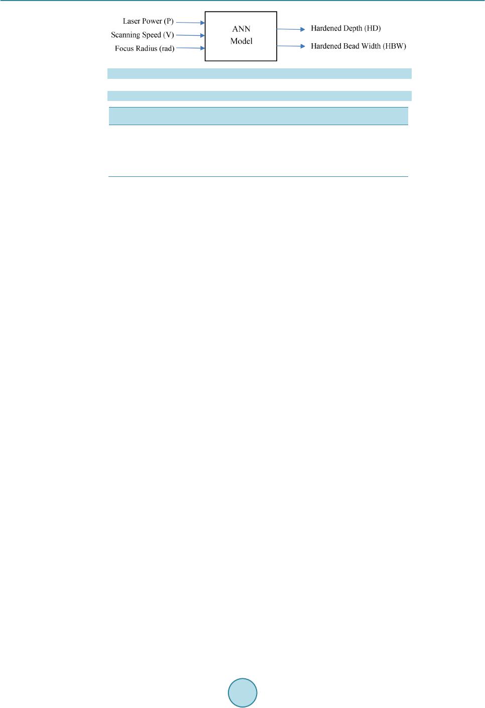 G. Billaud et al. Figure 13. Principle of the neural network. Table 8 . Middle points. Factors Factor Levels Laser Power (P) [W] 465 575 685 Scanning Veloci ty (V) [mm/s] 14 17 19 Focus Radius (Rad) [µm] 515 581.5 638 6.2. Result and Inte rp reta t ion Once the training step of the network is performed, the 27 combinations of verification data are applied as input parameters. The outputs of the ANN model are compared with those obtained by simulation. Therefore, this comparison is effective using various statistical indexes that characterize the prediction capability of the ANN model. Two main criteria are used to evaluate the accuracy of the network: the absolute error and the relative error. Figure 14 shows the a bso lute err or s for bo th HD and HB W for all 27 te st co mbinatio ns. The maxi mum ab so- lute errors for HD and HBW are, respectively, 64 and 94 µm. This means that the absolute error is of less than 100 µm for the overall test data, for both HD and HBW. Given that the values of HD are between 700 µm and 1100 µm, and that the values of HBW are between 2400 µm and 3000 µm, the model exhibits a good potential in terms of accuracy. As can be seen in the Figure 15, the relative errors for both the HD and HBW are very low in every case. The maximum relative errors for HD and HBW are, respectively, 8.01% and 3.62%. The mean relative errors for HD and HBW are 2.40% and 1.63%, re s pect ively, which he i ghtens the accuracy of the ne ural ne twork. Figure 16 and Figure 17 present, respectively, the results of the ANN models during the verification stage for HD and HBW. In fact, the figures show the ANN model and those obtained by simulation. The data are mostly located around the bisector of the 1st quadrant, which outlines the accuracy of the model. The two figures show that the net work is well tr ained and is hig hly effic ient. T he net work is t here fore a reliab le way to p red ict the HD and HBW for any combination of input parameters within the training range (between 480 W and 663 W for power, 12 mm/s and 20 mm/s for scanning velocity, 480 mm and 663 mm for focus radius). The ANN models don’t require any computation time to predict the outputs comparatively to the simulation. Note that the ANN models can predict the desired o utputs in the studied variation range only and they cannot extrapolate outside. Table 9 shows the comparison between the results generated by simulation and those generated by ANN model during training stage and confirms the observations from Figure 14 and Figure 15. Even if the ANN models have good performances in terms of robustness and accuracy, it is still important to validate them usi ng experimental validatio n. 7. Experimental Validation of the Neural Net wo r k The great number of data that can be generated by a 3D FEM allows to accurately train a neural network that will be able to predict the HD and HBW, and thus, it avoids the need to produce expensive experimental data that are often less numerous because of their cost. Once the network accuracy is verified with data generated by a FEM si mulation, experimental validation tests are conducted using a Nd:Yag laser and the shadowgraph measurement method. Eight sets are randomly chosen among the 27 sets of verification data. The experimental matrix is displayed in Table 10. The input powers are between 465 W and 685 W, the scanning velocities are between 14 mm/s and 17 mm/s. Finally, the focus radii are between 515 µm and 638 µm. 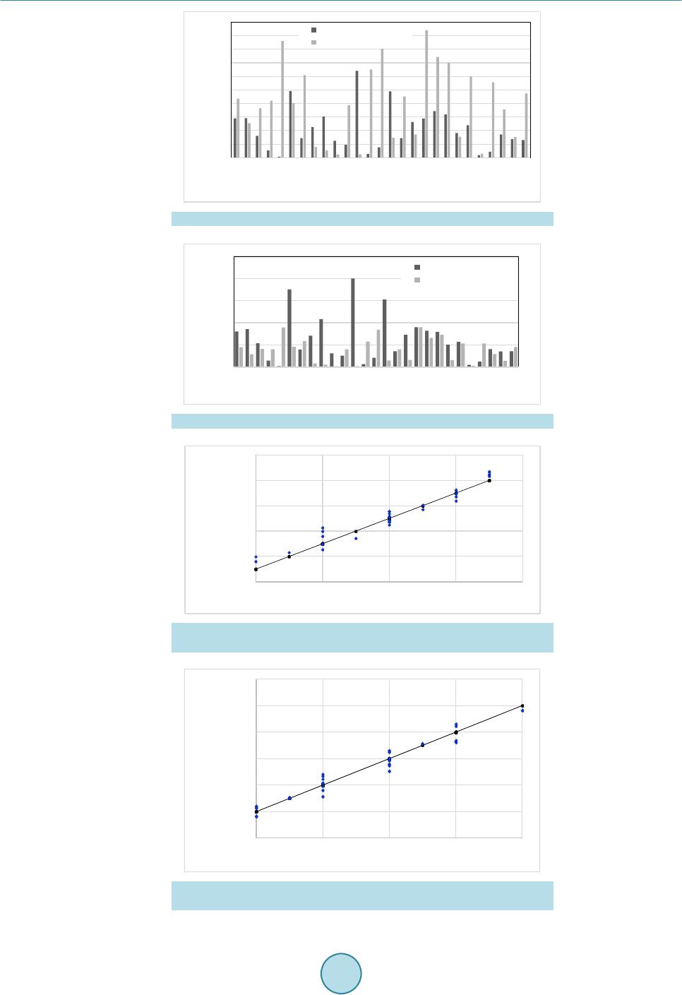 G. Billaud et al. Figure 14. Absolute relative errors for HD and HBW. Figure 15. Relative errors for HD and HBW. Figure 1 6. Comparison between simulated HD and HD calculated by the neural network. Figure 17. Comparison between simulated HBW and HBW calculated by the neura l ne t work . 650 750 850 950 1050 1150 7008009001000 1100 Predicted HD by neural network (µ m) 2000 2200 2400 2600 2800 3000 3200 2200 2400 2600 2800 3000 Predicted HBW by neural network ( µm)  G. Billaud et al. The results of the tests are shown in Table 11. The maximum relative errors for both the HD and HBW are 7.37% and 2.93%, respectively. The ANN is able to correctly predict both HD and HDW. It can now be used independently from the COMSOL software. It is easier to use as one only needs to compute the process parameters (within the training ranges of the ANN ) to obtain re lia ble results instantly. 8. Conclusion In this paper, a structured and comprehensive approach developed to design an effective ANN-based model for quality assessment and prediction in LSTHP using a commercial 3 kW Nd:Yag laser is presented. Several laser hardening parameters and cond itions were analyzed and their correlation with multiple performance characteris- tics of hardened surface was investigated using a structured experimental investigations and exhaustive 3D FEM Table 9. Comparison of the results. Simulation ANN mo dels Absolute error Relative error HD (µm) H BW (µm) HD (µm) HBW (µm) HD (µm) HBW (µm) HD (%) HBW ( %) Training Min 7 00 2000 698 2058 2 58 0.03 0.05 Max 1200 3200 1175 3147 25 53 4.88 4.52 Mea n 937 2557 931 2570 15 39 1.62 1.55 Verification Min 7 00 2200 730 2164 1 2 0.10 0.09 Max 1050 3000 1084 2964 64 94 8.01 3.62 Mea n 894 2522 902 2521 21 40 2.40 1.63 Table 10. Experimental matrix for validation. Test Powe r (W) Scanning velocity (mm/s) focus radius (µm) 1 465 14 515 2 575 19 515 3 685 17 515 4 685 14 515 5 575 14 581.5 6 685 17 581.5 7 465 17 638 8 685 17 638 Table 11. Experimental validation-results. Test Network HD (µm) Exp er imenta l HD (µm) Relative error for HD (%) Network HBW (µm) Experimen tal HB W (µm) Relative error for HBW (% ) 1 929 909 2.21 2444 2375 2.88 2 864 894 3.35 2302 2320 0.76 3 968 953 1.59 2470 2402 2.83 4 1084 1010 7.37 2726 2653 2.74 5 997 1018 2.04 2735 2702 1.22 6 952 1022 6.86 2603 2591 0.46 7 777 785 0.98 2392 2324 2.93 8 936 1002 6.55 2715 2643 2.73  G. Billaud et al. simulations under consistent p ractical pro cess conditions. Fo llowing the identi fication of the harden ing parame- ters and conditions that provide the best information about the LSTHP operation, tow type of modeling tech- niques were proposed to assess and predict the hardened bead width and hardened depth (HD) of the laser transformation hardened AISI 4340 steel plate: multiple regression analysis and ANN approach. The results demonstrate that the regression approach can be used to achieve a relatively accurate predicting model with cor- relation larger than 90%. The ANN models present greater results. The maximum relative errors for both HD and HBW are less than 8% an d 3%, respectively. Globally, the performance of the ANN-based model for qual- ity estimation and prediction in LSTHP shows significant improvement as compared to conventional methods. With a glob al maxi mum relative error less than 10% under various LSTHP conditions, the modeling procedure can be considered efficient and have led to conclusive results, due to the complexity of the analyzed process. The proposed approach can be effectively and gainfully applied to quality assessment for LSTHP, because it in- cludes the advantages of ease of application, reduced modeling time and sufficient modeling accuracy. References [1] Kannat ey-Asibu , E. (2009) Principles of Laser Materials Processing. Wiley, Hoboken. http://dx.doi.org/10.1002/9780470459300 [2] Steen, W.M. (2010) Laser Material Pro cess ing. 4th Edition, Springer, London. http://dx.doi.org/10.1007/978-1-84996-062-5 [3] Patwa, R. and Shin, Y.C. (2007) Predictive Modeling of Las er Harden ing of AISI5150H Steels. International Journal of Machine Tools and Manufacture, 47, 307-320. http://dx.doi.org/10.1016/j.ijmachtools.2006.03.016 [4] Mioković, T., Schulze, V., Vöh ringer, O. and Löhe, D. (2006) P rediction of Phase Trans formations during Laser Sur- face Harden in g of AISI 4140 including the Effects of Inhomogeneous Austenite Formation. Materials Science and En- gineer ing: A, 435-436, 547-555. http://dx.doi.org/10.1016/j.msea.2006.07.037 [5] Ashby, M.F. and Easterling, K.E. (1984) The Transformation Hardening of Steel Surfaces by Laser Beams—I. Hyp o- Eutect oid Steels . Acta Metallurgica, 32, 1935-1948. http://dx.doi.org/10.1016/0001-6160(84)90175-5 [6] Antony, J. and Jiju Antony, F. (2001) Teaching the Taguchi Method to Industrial Engineers. Work Study, 50, 141-149. http://dx.doi.org/10.1108/00438020110391873 [7] Chen, S.L. and Sh en, D. (1999) Optimisation and Quantitative Evaluation of the Qualities for Nd-YAG Laser Trans- formation Hardening. International Journal of Advanced Manufacturing Technology, 15, 70-78. http://dx.doi.org/10.1007/s001700050041 [8] Badkar, D., Pandey, K. and Buvanash ekaran, G. (2011) Parameter Optimization of Laser Transformation Hardening by Using Taguchi Method and Utility Concept. International Journal of Advanced Manufacturing Technology, 52, 1067- 1077. http://dx.doi.org/10.1007/s00170-010-2787-z [9] Benyounis, K.Y., Olabi, A.G. and Hashmi, M.S.J. (2005) Effect of Laser Welding Parameters on the Heat Input and Weld-Bead Profile. Journal of Materials Processing Technology, 164-165, 978-985. http://dx.doi.org/10.1016/j.jmatprotec.2005.02.060 [10] Sathiya, P., Abdul Jaleel, M.Y. and Katherasan, D. (2010) Optimization of Welding Parameters for Laser Bead-on- Plate Welding Using Taguchi Method. Production Engineering-Research and Development, 4, 465-476. http://dx.doi.org/10.1007/s11740-010-0234-5 [11] Hagan, M.T., Demuth, H.B. and Beale, M.H. (1996) Neural Network Design: Pws Boston. [12] Ciurana, J., Ar ias , G. and Ozel, T. (2009) Neural Net work Modelin g and Particle S warm Optimi zation (P SO) of Proc- ess Parameters in P ulsed Laser Micromachinin g of Hardened AI SI H13 Steel . Materials & Manufacturing Processes, 24, 358-368. http://dx.doi.org/10.1080/10426910802679568 [13] Pan, Q.Y., Huang, W.D., Song, R.G., Zhou, Y.H. and Zhang, G.L. (1998) The Improvement of Localized Corrosion Resistance in Sensitized Stainless Steel by Laser Sur fac e Remelting. Surface and Coatings Technology, 102, 245-255. http://dx.doi.org/10.1016/S0257-8972(98)00358-2 [14] Munteanu, A. (2012) Surface Hardness Prediction Using Artificial Neural Networks in Case of Electron Beam Ma- chining Process. Romanian Association of Nonconventional Technologies. [15] Doane, D. (1979) Applica ti on of Hardenability Concepts in Heat Treatment of Steel. Journal of Heat Treating, 1, 5-30. http://dx.doi.org/10.1007/BF02833206 [16] Haykin, S. (2010) Neural N etworks: A Comprehensive Foundation, 1994. Mc Millan, New Jersey. [17] Principe, J., Euliano, N. and Lefebvre, W. (2000) Neural and Adaptive Systems: Fundamentals through Simulations. John Wiley and Sons, New York.
|