Journal of Electromagnetic Analysis and Applications
Vol.5 No.1(2013), Article ID:27315,11 pages DOI:10.4236/jemaa.2013.51006
Electromagnetic Oscillations in a Spherical Conducting Cavity with Dielectric Layers. Application to Linear Accelerators
![]()
1Institute of Physics, Polish Academy of Sciences, Warsaw, Poland; 2Department of Theoretical Physics, National Centre for Nuclear Research, Warsaw, Poland.
Email: wladyslaw.zakowicz@ifpan.edu.pl, askor@fuw.edu.pl, einfeld@fuw.edu.pl
Received November 11th, 2012; revised December 12th, 2012; accepted December 20th, 2012
Keywords: Spherical Cavity; Spherical Dielectric Layer; TE Mode; TM Mode; Q Factor; Linear Accelerator
ABSTRACT
We present an analysis of electromagnetic oscillations in a spherical conducting cavity filled concentrically with either dielectric or vacuum layers. The fields are given analytically, and the resonant frequency is determined numerically. An important special case of a spherical conducting cavity with a smaller dielectric sphere at its center is treated in more detail. By numerically integrating the equations of motion we demonstrate that the transverse electric oscillations in such cavity can be used to accelerate strongly relativistic electrons. The electron’s trajectory is assumed to be nearly tangential to the dielectric sphere. We demonstrate that the interaction of such electrons with the oscillating magnetic field deflects their trajectory from a straight line only slightly. The Q factor of such a resonator only depends on losses in the dielectric. For existing ultra low loss dielectrics, Q can be three orders of magnitude better than obtained in existing cylindrical cavities.
1. Introduction
It has been shown [1-3] that, if a plane electromagnetic wave is scattered on a finite dielectric object, structural resonances can be excited in the object (e.g., whispering gallery modes). They are associated with very high amplitudes of oscillating EM fields in the dielectric and its vicinity. Their maxima exceed values reached in resonant cavities of typical linear accelerators by several orders of magnitude. Therefore, one can think of applying these fields to accelerate charged particles [1-3]. Many other applications of the whispering gallery modes are described in [4-6].
As for the proposals given in [1-3], both light produced by lasers and microwaves are conceivable. However, it is difficult to achieve the required synchronization of wave particle in the optical frequency range. In the microwave frequency range, this mechanism would require excessive total excitation energy and so may not be practical.
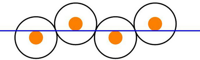
In this paper we demonstrate that the last mentioned problem can be overcome by locating the dielectric object in a resonant cavity. This appeals to traditional accelerating structures used in SLAC, see Figure 1. In the latter case, maximum amplitudes of accelerating fields are restricted by Joule heating losses in conducting walls and electric breakdown. In this connection, in existing accelerators (e.g., in LHC) one avoids sharp edges of the walls and uses superconductive resonant
 (a)
(a)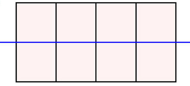 (b)
(b)
Figure 1. Proposed multi cell accelerator units (a) vs. those of SLAC (b), assuming the same electron transit time through the cavity.
cavities. Unfortunately, since superconductivity of the walls disappears if the magnetic field on the wall exceeds a critical value, the maximal values of accelerating fields in these highly complicated cavities are not much higher than those reached in SLAC.
The presence of a dielectric in the central part of the resonance cavity shifts the magnetic field maximum from regions close to the metallic wall towards the dielectric surface. This considerably lowers skin effect losses in the wall. Even though additional losses due to dielectric heating are introduced, total losses would nevertheless be lower if one could apply ultra low loss dielectrics (with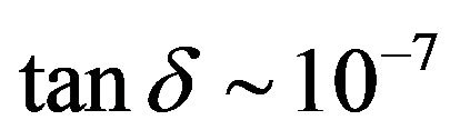 ) as described in [7,8]. In that case, a resonator quality reaching
 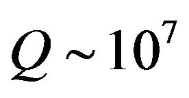 can be obtained, as compared to
  for SLAC.
2. A Spherical Conductive Cavity with Dielectric Layers
Our approach to describe electromagnetic oscillations in a resonant cavity assumes that the cavity can be divided into regions in which the fields can be determined analytically. The resonant frequency is defined by the fact that the fields must satisfy boundary conditions at the cavity wall along with continuity conditions at the interfaces. This frequency will be determined by numerically solving the consistency condition for these requirements.
In general, we assume that the cavity is bounded by a conducting spherical surface, and filled concentrically with  either dielectric or vacuum layers. Each dielectric layer is assumed to be homogeneous. We introduce a spherical coordinate system
  with its origin at the cavity center. The layers are bounded by
 , up to
  for the metallic boundary, see Figure 2.
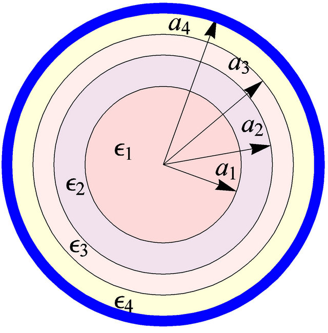
Figure 2. An example of a spherical cavity with dielectric layers (N = 4).
The harmonically oscillating electromagnetic fields in each concentric layer are described by Maxwell’s equations (Gaussian units, magnetic permeability , and complex fields proportional to
 ):
):
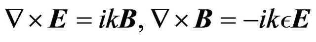 (1)
(1)
where
 (2)
(2)
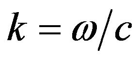
 is the angular frequency, and
  denotes complex dielectric permittivity
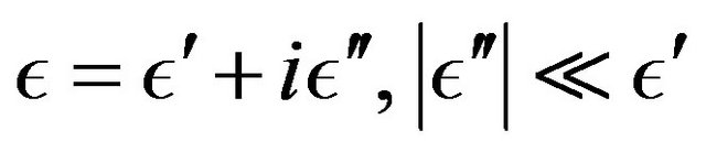 (3)
(3)
These fields split into transverse electric (TE) or transverse magnetic (TM), which have no radial components of either field [9]. In an ideal resonator with perfectly conducting walls and perfect dielectrics, pure TE or TM modes can be excited. They will also be approximately valid in real resonators if their energy losses are not too high.
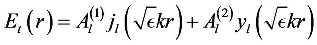
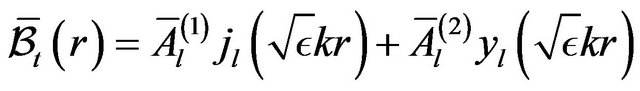
Using (9.116), and (9.119) in [9], which describe the vacuum TE field in spherical coordinates, and replacing there  we obtain the most general form of the TE field in the uniform dielectric:
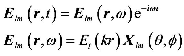 (4)
(4)
where
 (5)
(5)
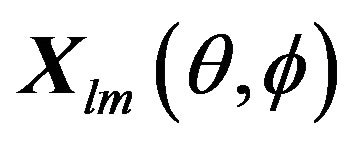 are vector spherical harmonics as defined by Eqation (9.119) in [9], and
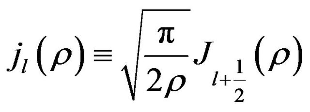
and 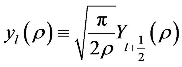
are spherical Bessel and Neumann functions.
The corresponding magnetic induction can be determined from the first Maxwell Equation (1). Using also (10.60) in [9] we obtain
 (6)
(6)
where  involves both the transverse and radial component:
 (7)
(7)
in which
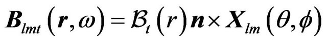 (8)
(8)
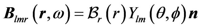 (9)
(9)
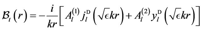 (10)
(10)
 (11)
(11)
Here  are spherical harmonics,
  ,
,  is a positive integer related to the integer
  by
by 
and 
are derivatives of the Riccati-Bessel and Riccati-Neumann functions.
In a similar way, using (9.118), (9.119) and (10.60) in [9] along with the second Maxwell Equation (1), we obtain for the TM modes in the uniform dielectric:
 (12)
(12)
where
 (13)
(13)
 (14)
(14)
where  involves both the transverse, and radial component:
 (15)
(15)
in which
 (16)
(16)
 (17)
(17)
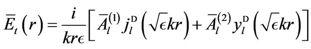 (18)
(18)
 (19)
(19)
In our analysis we will admit small energy losses in both the wall and the dielectric layers. However, when calculating the resonant frequency of the cavity , these losses will be neglected. Thus the wall is assumed to be perfectly conducting. This means that it carries no electric or magnetic field. Then continuity of the tangential components of the electric field and the normal components of the magnetic induction at each interface require vanishing of these components at the boundary of
  th layer at
 . In view of (4)-(9), and (12)-(19) this will be the case if the following boundary conditions at
  are fulfilled:
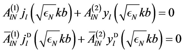 (20)
(20)
where the upper line refers to TE modes and the lower one to TM modes.
In the first layer which contains the origin  we must choose
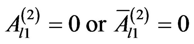 (21)
(21)
to avoid singularities of  or
or  at
at .
.
In the simplest case of a spherical cavity filled completely with the dielectric (or vacuum), i.e.,  , the boundary conditions (20) lead to
 (22)
(22)
where  This defines the resonant frequency
  of either TE or TM modes, depending only on
  and
and .
.
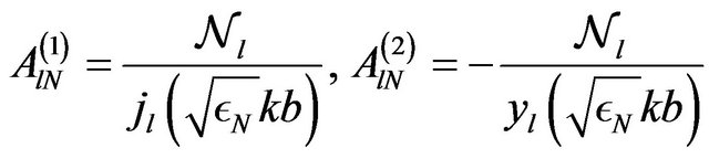
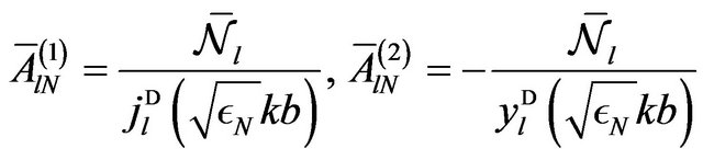
In the presence of layers ,
,  must also depend on
 etc. and therefore condition (22) cannot be fulfilled. In fact, for the same reason, we can assume that also the remaining functions in conditions (20) are non-vanishing. Therefore these conditions can be satisfied by choosing
 (23)
(23)
 (24)
(24)
for TE modes (upper line) or TM modes, where  and
and  are normalization factors.
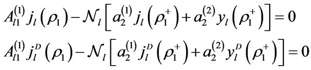
At the interfaces between dielectrics, the following quantities must be continuous: the tangential components of the electric field and normal ones of the magnetic induction and furthermore, the tangential components of the magnetic induction, due to vanishing of the surface currents at the dielectric surface. For the TE modes, this leads to the following conditions at 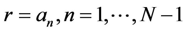 :
:
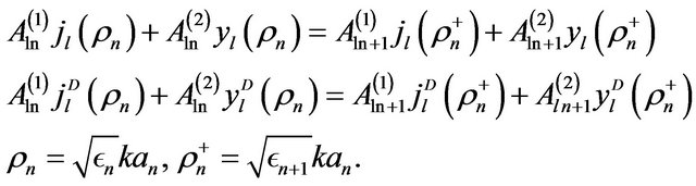 (25)
(25)
This can be written in matrix form
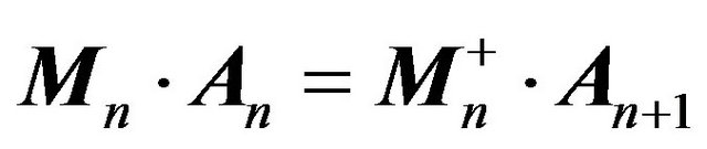 (26)
(26)
where
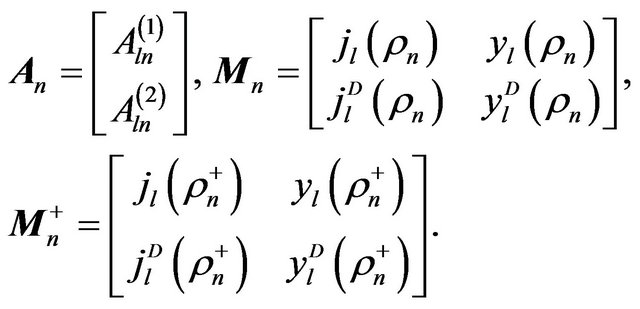 (27)
(27)
The  matrices are non-singular:
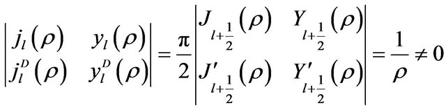 (28)
(28)
where last equality follows from the fact that  and
and  are solutions of the Bessel equation

Multiplying (26) by
 (29)
(29)
we arrive at the recurrence relation
 (30)
(30)
For the  th interface between dielectrics, this relation defines the vector
  at the lower layer in terms of that at the upper one. Using this relation successively for
 , we can express all
  vectors in terms of
 (31)
(31)
i.e.,
 (32)
(32)
We recall that in the first layer we must satisfy , see (21). In view of this requirement, Equation (25) for
  can be written as
 (33)
(33)
where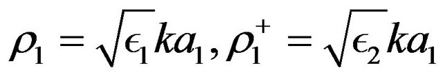 , and
, and 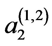 are components of the vector
 . This vector is defined by (32) and (31) if
 :
:
 (34)
(34)
For ,
,  is defined by (31), i.e., is given by the last factor in (34).
The linear and homogeneous set of Equation (33) for  and
and  will have non-zero solutions if and only if its determinant vanishes,
 (35)
(35)
If this condition is fulfilled,  is given by either of Equation (33), which are equivalent. Like all remaining coefficients
  and
and , also
  will be proportional to the normalization factor
 , see (32) and (33).
If there are only two layers ,
,  and
and  in (33) and (35) are given by (31) and the resonant frequency
  defined by (35) can be found from
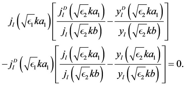 (36)
(36)
and
 (37)
(37)
By replacing in (25)-(37)
 (38)
(38)
for any  and
and , we obtain the corresponding equations for the TM modes.
Any standard software like Mathematica or Maple can be used to solve the non-linear Equations (35) or (36) defining the resonant frequency , along with the pertinent linear algebra for
 . We did it for
 , see the following section, and also for
 , by using Mathematica.
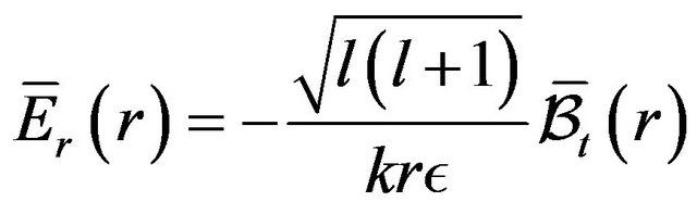
Note that for the TM modes, where  in (19) is continuous at each dielectric interface,
  will have jumps, due to discontinuities in
 . However, the radial component of the electric displacement
 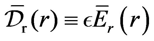 will be continuous. This will also be true of the TE modes where the radial displacement is identically zero. These facts imply the vanishing of surface charges at each dielectric interface. And this in turn means that the multi-layer dielectric structure resembles (and can approximate) a smooth dielectric with some permittivity profile
 , in spite of jumps in
 .
.
It was pointed out to us by Paul Martin of SIAM, that our matrix Equation (26), which can be used to relate the EM fields of a given mode for two layers of a stratified sphere, is not new. It was probably first used by A. Moroz [10] when calculating forced oscillations in such a sphere but without a conducting wall, induced by an oscillating electric dipole. In this application, the frequency  is arbitrary.
3. A Spherical Conductive Cavity with a Dielectric Sphere
The general theory given in the previous section will now be illustrated by calculations pertinent to the TE modes in a spherical cavity with a dielectric sphere of radius  and dielectric permittivity
 , i.e., for
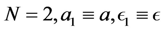 , and
, and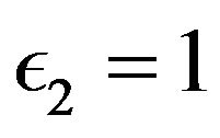 .
.
Fields in such a system will be described by Equations (4)-(9) both in the sphere and the surrounding vacuum. In view of (21) and (23) their radial profiles will be given by
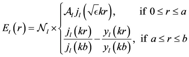 (39)
(39)
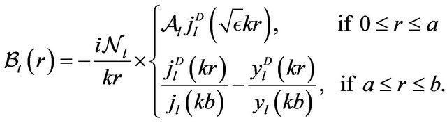 (40)
(40)
Replacing 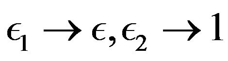 and
and 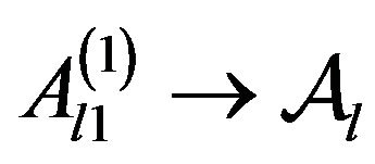 in (36) and (37), we obtain equations defining the resonant frequency
  and the amplitude coefficient
 .
.
We verified that for , the average energies associated with the electric and the magnetic field in the cavity are equal:
 (41)
(41)
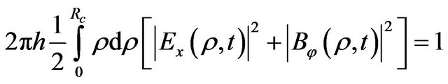
(This was a check on the correctness of our formulas and accuracy of calculations.) The normalization constant  was chosen so as to satisfy:
 (42)
(42)
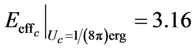
(The corresponding average energy associated with the electric and the magnetic field over our cavity is  erg.)
erg.)
In Figure 3,  as a function of
  is presented for three spherical cavities with dielectric spheres. Note that
  is
is  independent (due to degeneracy). This fact is one of the reasons why the spherical resonator shown in Figure 1 cannot be used in the final project of a real accelerator even though it is very convenient for a general analysis. The degeneration in question can be broken e.g., by replacing the spherical resonator by an ellipsoidal one, or shifting the center of the dielectric sphere. Another possibility could be to use an anisotropic dielectric. In any case, however, a separate numerical analysis would be necessary.
In Figure 4 we give an example of radial functions in the equations describing fields in our spherical cavity with a dielectric sphere, (4), (8) and (9). Large values of these functions in a vicinity of the dielectric boundary can be observed.
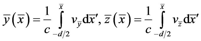
3.1. The Motion of Relativistic Electrons
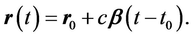
The trajectory  of a relativistic electron crossing the spherical cavity shown in Figure 1 can be parametrized by the electron's closest approach
  and electron velocity
 :
:
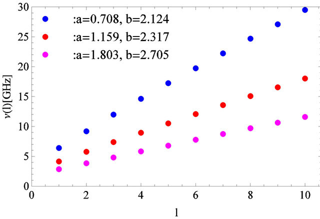
Figure 3. The resonant frequencies  vs.
vs.  for three spherical cavities with dielectric spheres (
 and
and  in cm). Note that
  is
is  independent (due to degeneracy).
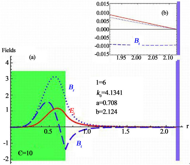
Figure 4. (a) Field radial functions for a spherical cavity with dielectric sphere and perfect metallic wall (Gaussian units,  ,
,  and
and  in cm). And the complete fields are given by (4)-(11). Note that
  and
and  vanish at the wall, whereas
  is non-zero but small, see (b).
 (43)
(43)
The origin of the Cartesian coordinate system  was chosen at the center of the dielectric sphere, and the electron moving along the
  axis was passing just above the dielectric sphere as shown in Figure 1. We chose
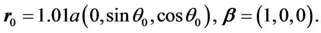 (44)
(44)
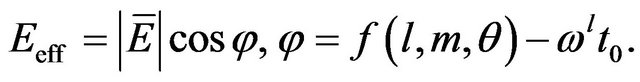
The effective accelerating field felt by the electron as it passes through the cavity,  , is equal to the real part of
 (45)
(45)
where  is the electron trajectory segment within the cavity,
  is the
  component of the electric field
  given by (4) and
  is given by (43). Thus
 (46)
(46)
Maximal acceleration is obtained if
if  is chosen so that the accelerating phase
 . With this choice, the relativistic electron is never decelerated within the spherical cavity, see Figure 5, where two examples are given. Typical results for
  obtained with our normalization (42) are shown in Figures 6 and 7.
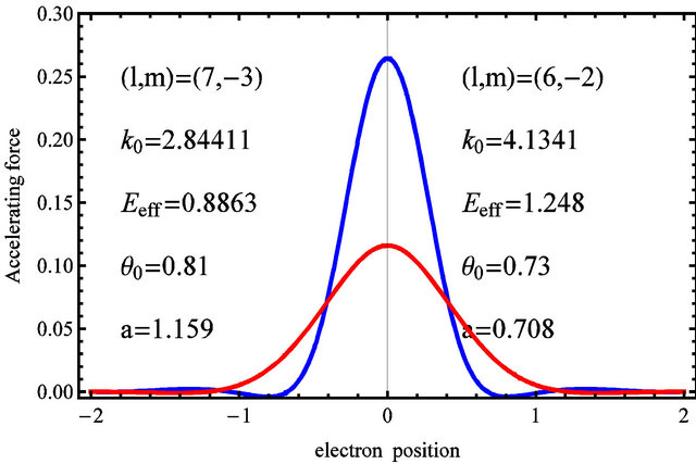
Figure 5. The accelerating force (in units of  dyne) acting on an electron as it moves through the cavity shown in Figure 1 (
 ,
, in kV/m, and dimensions in cm).
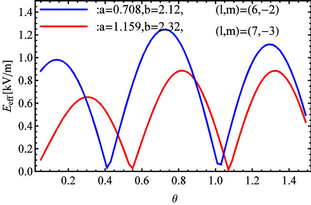
Figure 6. Effective accelerating field as a function of  for two spherical cavities (
 and
and  in cm).
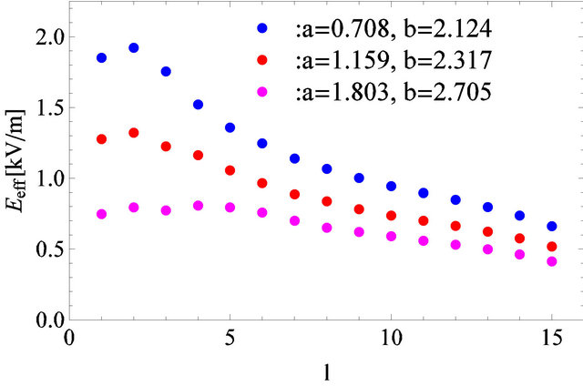
Figure 7. Effective accelerating fields vs.  for three spherical cavities with the assumed normalization of the RF field, see (42) (
 and
and  in cm). For each value of
 , these values were optimized with respect to
  as well as
 , see Figure 6.
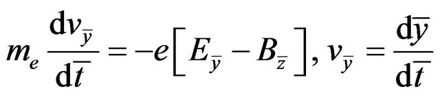
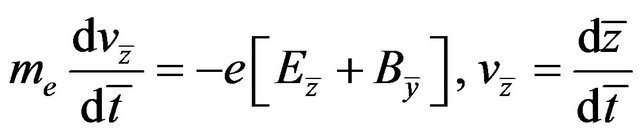
The electromagnetic field given by the real parts of (4), (8) and (9) is strongly non-uniform. Therefore one should check how much the relativistic electron will deflect from the assumed trajectory  given by (43), due to interaction with this field. A nice feature of our model is that the field in question is described analytically by (4)-(9) so that the pertinent equations of the transversal motion can easily be integrated numerically.
In a real accelerator, where we are dealing with an electron beam of finite cross section, the electromagnetic fields  and
and  acting on each electron will be superpositions of the external fields and the fields due to the electron charge and current. However, in the lowest approximation (and particularly for not too large beam densities) the latter fields can be neglected. Furthermore, if as in our case, the transversal deflections are small, the deflecting fields can be calculated on the unperturbed trajectory given by (43). It will also be assumed that the electron mass
 , is time independent within the spherical cavity. With these approximations, and within the Cartesian coordinate system
  with its center at
 , the
, the  axis along the unperturbed trajectory, and the
  axis along
 , the electron’s transversal motion will be described by
 (47)
(47)
 (48)
(48)
where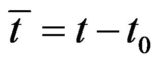 , the field components
 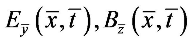 , etc. are given by the real parts of Equations (4), (8) and (9), taken at
 , and
, and . Integrating these equations with zero initial conditions we end up with
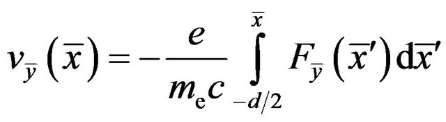 (49)
(49)
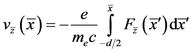 (50)
(50)
 (51)
(51)
where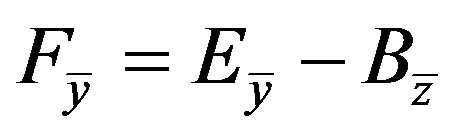 , and
, and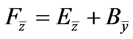 .
.
In Figures 8 and 9 we give an example of the coordinates  and
and  of the deflecting force. They correspond to
  cm,
cm,  cm, and
 , for which the the accelerating field will be our reference value
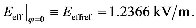 (52)
(52)
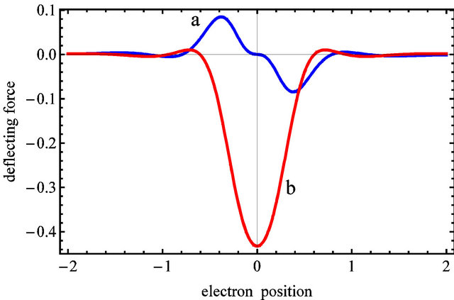
Figure 8. The deflecting force coordinate  for the accelerating phase
  (a) and
  (b), see Figure 5 for units and parameters (right column).
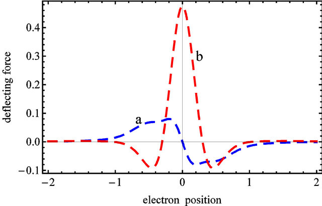
Figure 9. The deflecting force coordinate  for the accelerating phase
  (a) and
  (b), see Figure 5 for units and parameters (right column).
It can be seen that if the accelerating phase , both
  and
and  are odd functions. Therefore in this case of maximal acceleration, there will be no transversal velocity increments over the cavity,
  . At the same time the velocity components
  and
and  in (51) will be even functions of
  tending to zero as
 . Hence the transversal deflections
  and
and  will be increasing functions tending to constants as
 , see Figure 10(a).
For the worst case of accelerating phase  for which
  and
and  will be increasing functions soon reaching their limiting values
  and
and  for
for . The corresponding transversal motions
  and
and  will soon become uniform for
 , leading to much larger deflections at
 , see Figure 10(b).
The actual transversal deflections per cavity in an accelerator involving our spherical cavities can be obtained by multiplying the normalized values given in Figure 10 by the factor
 (53)
(53)
where  is given by (52),
  is the assumed value of the effective accelerating field, and
 . For large values of
 , small
  requires
  to be sufficiently large. Assuming that
  , see Figure 10(a) is not larger than
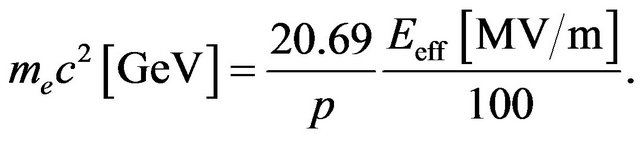
  of the spacing between the dielectric sphere and the electron trajectory,
  cm, the required minimal electron energy is given by
 (54)
(54)
Thus, if we assume that  MV/m, the transversal displacements will be smaller than
 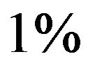 of the spacing in question, if the electron energy
 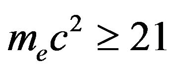 GeV, i.e., for typical output energies from SLAC. Whether the real dielectric can withstand this value of
  is another question beyond the scope of this paper. More comments will be given later on.
3.2. Quality Factors
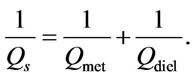
An important parameter of any linear accelerator is the quality  of its resonant cavities:
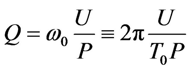 (55)
(55)
where  is the resonant angular frequency of the ideal cavity
 ,
,  is the corresponding reso-

Figure 10. Conveniently normalized transversal displacements  (solid curves) and
  (dashed curves) as functions of
  for the accelerating phase
  (a) and
  (b), see Figure 5 for units and parameters (right column).
nant period,  is the time-averaged energy stored in the cavity
 (56)
(56)
and  is time-averaged cavity power loss.
The power loss caused by the skin current in the metallic wall bounded by the surface  is given by
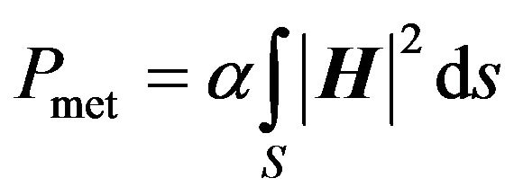 (57)
(57)
where
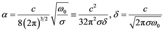 (58)
(58)
 is the skin depth,
  is conductivity of the wall, and the magnetic field intensity
  refers to the ideal cavity, i.e., its normal component is vanishing
 .
.
The quality of the cavity related to losses in the metallic wall is thus given by
 (59)
(59)
Using the fact that at resonance, the averaged energies stored in the electric and magnetic fields are equal, see (41), we end up with :
:
 (60)
(60)
This formula is quite general, and in particular can also be used for a traditional cylindrical cavity of radius  and height
 . In that case, the cylindrically symmetric
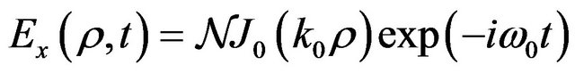
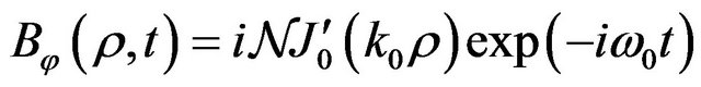
  TM mode used for acceleration is given by
 (61)
(61)
 (62)
(62)
where ,
,  is a Bessel function, and
  and
and  are cylindrical coordinates (cylindrical axis along
 ).
).
The vanishing of  on an ideally conducting cylindrical wall requires that
 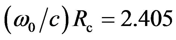 (the smallest zero of
 ) which defines the angular resonant frequency in terms of
 . Equations (62) and (60) lead to the well known formula for the quality of the cylindrical pill box cavity
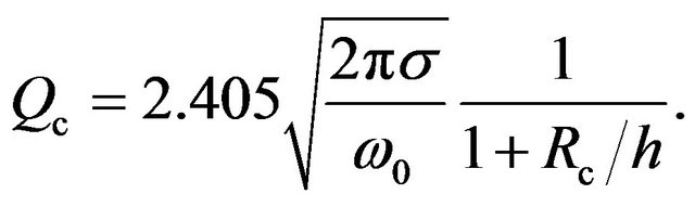 (63)
(63)
For the SLAC pill box cavity shown in Figure 1 (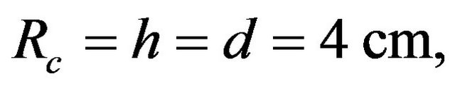 and
and  for copper wall in room-temperature), this formula leads to
 . The corresponding values for spherical cavities with ideal dielectric spheres and the same values of
  and
and  reach much larger values, see Figure 11.
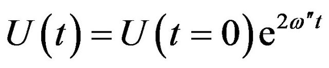
In the presence of the dielectric sphere, one is also dealing with losses due to an imperfect dielectric specified by . The non-vanishing value of
  leads to
 , for
, for  defined by (35). In view of Equation (2) this implies a complex value of
 .
.
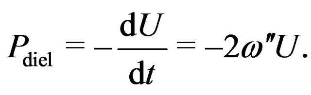
For the fields given by (4)-(9), we obtain
where  for the energy
  being dissipated rather than generated. Using this result we find for the power losses in the dielectric:
In view of (55), the corresponding quality will thus be given by
 (64)
(64)
This value is of the order of . It is approximately
  independent.
In our calculations we took  and
and . Dielectrics with such ultra small losses were investigated in [8].
The total power loss in the spherical cavity encasing the dielectric sphere  is due to the power loss in the metallic wall and that in the dielectric sphere:
 (65)
(65)
Dividing both sides of this relation by  and using (55) we obtain
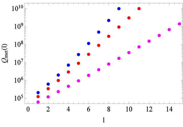
Figure 11. The quality  vs.
vs.  for three spherical cavities with ideal dielectric spheres (see Figure 7).
 (66)
(66)
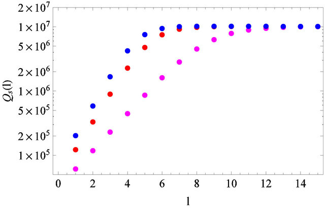
where  is the total Q-factor of the spherical cavity. Values of
  versus
  for three spherical cavities with dielectric spheres and
  cm are shown in Figure 12. They are about three orders of magnitude larger than
 .
.
In a real accelerator, openings in the metallic wall are necessary for free penetration of the cavity by the electron beam, and to enable coupling between neighboring cavities. This will lower the quality  but should have little effect on the total quality of the spherical cavity
 . The latter is defined by losses in the dielectric, see (66) where
 . The resonant frequency should not be drastically changed either, as the EM fields at the iris
 are very small fractions of their maxima, see Figure 4.
3.3. Discussion and Summary
When comparing the effective accelerating fields in the traditional pill box cavity with that in our spherical cavities with dielectric spheres, we first assume that , the time-averaged energy stored in the cavity, see (56), is the same in both situations. Therefore the normalization factor
  in (61) and (62) will first be chosen so that
 (67)
(67)
see (42) ( erg).
erg).
The complex effective accelerator field  for the cylindrical resonator shown in Figure 1
 is given by the right hand side of (45) in which
  is defined by (61) with
 , and
, and . The result is
 (68)
(68)
 vs.
vs.  for three spherical cavities with dielectric spheres (see
 where  is the time at which the electron passes the center of the cavity.
We now denote by  and
and  the maximal effective accelerating fields (equal to
 ) for the spherical cavity with a dielectric sphere and the traditional cylindrical cavity, for any values of the average energies in the cavities,
  and
and . In view of the fact that
  in (61) is proportional to
  we can write, using the definition (55) of
 ,
,
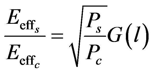 (69)
(69)
where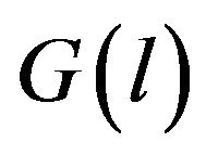 , the “gain factor”, is given by
 (70)
(70)
Here  and
and  are the resonant frequencies of the spherical and the cylindrical cavities
  and
and  and
and  are the corresponding power losses. They are equal to the powers that must be supplied from external sources to sustain the oscillations. They should be as large as possible to avoid breakdown in the dielectric or at the metallic wall. Further research is necessary to give an estimate of the ratio
 . We can only hope that it is not smaller than unity.
For our typical SLAC pill box cavity shown in Figure 1  we obtain
  and
and
 kV/m to be used in (70). The resulting values of the gain factor are shown in Figure 13.
The results of our calculation are shown in Figures 3-13 for three reasonable values of
 .
.
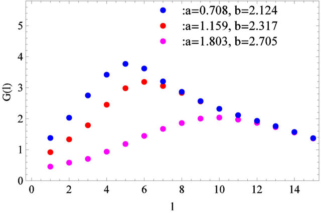
Figure 13. Gain factor  in (69) and (70) for three spherical cavities (
 and
and  in cm).
The electron trajectory segment inside the cavity shown in Figure 1 was equal to the typical length of the pill-box cavity of SLAC (4 cm). Calculations were performed for various values of  and
and . The optimal parameters found were:
  cm,
cm,  cm, and
 .
.
4. Conclusion
An electric field, intensified by structural resonance, can be used to accelerate electrons. This is demonstrated here by placing a dielectric sphere concentrically inside a spherical resonator, in which an appropriate whispering gallery mode is excited. A strong, accelerating field appears next to the surface of the dielectric. At the same time, the tangential component of the magnetic field at the wall of the resonator is minimal. This makes losses at the metallic walls negligible without engaging expensive cryogenic systems ensuring superconductivity of the walls. The Q factor of the resonator only depends on losses in the dielectric. For existing dielectrics, this gives a Q factor three orders of magnitude better than obtained in existing cylindrical cavities. Furthermore, for the proposed spherical cavity, all field components at the metallic wall are either zero or very small, see Figure 4. Therefore, one can expect the proposed spherical cavity to be less prone to electrical breakdowns than the traditional cylindrical cavity.
5. Acknowledgements
The authors would like to thank Professor  Kuliński for useful discussions.
REFERENCES
- W. Zakowicz, “Whispering-Gallery-Mode Resonances: A New Way to Accelerate Charged Particles,” Physical Review Letters, Vol. 95, No. 11, 2005, Article ID: 114801. doi:10.1103/PhysRevLett.95.114801
- W. Zakowicz, “Erratum: Whispering-Gallery-Mode Resonances: A New Way to Accelerate Charged Particles [Phys. Rev. Lett. 95, 114801 (2005)],” Physical Review Letters, Vol. 97, No. 10, 2006, Article ID: 109901. doi:10.1103/PhysRevLett.97.109901
- W. Zakowicz, “Particle Acceleration by Wave Scattering off Dielectric Spheres at Whispering-Gallery-Mode Resonance,” Physical Review Special Topics—Accelerators and Beams, Vol. 10, No. 10, 2007, Article ID: 101301. doi:10.1103/PhysRevSTAB.10.101301
- M. Ornigotti and A. Aiello, “Theory of Anisotropic Whispering-Gallery-Mode Resonators,” Physical Review A, Vol. 84, No. 1, 2011, Article ID: 013828. doi:10.1103/PhysRevA.84.013828
- T. V. Liseykina, S. Pirner and D. Bauer, “Relativistic Attosecond Electron Bunches from Laser-Illuminated Droplets,” Physical Review Letters, Vol. 104, No. 9, 2010, Article ID: 095002. doi:10.1103/PhysRevLett.104.095002
- V. S. Ilchenko, A. A. Savchenkov, A. B. Matsko and L. Maleki, “Nonlinear Optics and Crystalline Whispering Gallery Mode Cavities,” Physical Review Letters, Vol. 92, No. 4, 2004, Article ID: 043903. doi:10.1103/PhysRevLett.92.043903
- R. C. Taber and C. A. Flory, “Microwave Oscillators Incorporating Cryogenic Sapphire Dielectric Resonators,” IEEE Transactions on Ultrasonics, Ferroelectrics and Frequency Control, Vol. 42, No. 1, 1995, pp. 111-119. doi:10.1109/58.368306
- J. Krupka, K. Derzakowski, M. E. Tobar, J. Hartnett and R. G. Geyer, “Complex Permittivity of Some Ultralow Loss Dielectric Crystals at Cryogenic Temperatures,” Measurement Science and Technology, Vol. 10, No. 5, 1999, pp. 387-392. doi:10.1088/0957-0233/10/5/308
- J. D. Jackson, “Classical Electrodynamics,” 3rd Edition, John Wiley, New York, 1998.
- A. Moroz, “A Recursive Transfer-Matrix Solution for a Dipole Radiating inside and outside a Stratified Sphere,” Annals of Physics, Vol. 315, No. 2, 2005, pp. 352-418. doi:10.1016/j.aop.2004.07.002