Int'l J. of Communications, Network and System Sciences
Vol.7 No.7(2014), Article ID:48126,8 pages
DOI:10.4236/ijcns.2014.77027
Buffer Management in the Sliding-Window (SW) Packet Switch for Priority Switching
Alvaro Munoz1, Sanjeev Kumar2
1Samsung Inc., Richardson, Texas, USA
2Department of Electrical and Computer Engineering, The University of Texas-Pan American, Edinburg, USA
Email: sjk@utpa.edu
Copyright © 2014 by authors and Scientific Research Publishing Inc.
This work is licensed under the Creative Commons Attribution International License (CC BY).
http://creativecommons.org/licenses/by/4.0/


Received 26 May 2014; revised 26 June 2014; accepted 12 July 2014
ABSTRACT
Switch and router architectures employing a shared buffer are known to provide high throughput, low delay, and high memory utilization. Superior performance of a shared-memory switch compared to switches employing other buffer strategies can be achieved by carefully implementing a buffer-management scheme. A buffer-sharing policy should allow all of the output interfaces to have fair and robust access to buffer resources. The sliding-window (SW) packet switch is a novel architecture that uses an array of parallel memory modules that are logically shared by all input and output lines to store and process data packets. The innovative aspects of the SW architecture are the approach to accomplishing parallel operation and the simplicity of the control functions. The implementation of a buffer-management scheme in a SW packet switch is dependent on how the buffer space is organized into output queues. This paper presents an efficient SW buffermanagement scheme that regulates the sharing of the buffer space. We compare the proposed scheme with previous work under bursty traffic conditions. Also, we explain how the proposed buffer-management scheme can provide quality-of-service (QoS) to different traffic classes.
Keywords: Sliding Windows Switch, Priority Switching, Buffer Management

1. Introduction
A shared-memory switch allows multiple high-data-rate lines to share a common buffer space for storing packets destined to various output ports of the switch. Switching systems employing shared memory have been known to provide the highest throughput and incur the lowest packet loss compared to packet switches employing input or output buffering strategies under conditions of identical memory size and bursty traffic [1] . In order for a shared-memory switch to achieve optimal performance, the memory-management algorithm must carefully control how the common buffer space is allocated among various output queues. The problem is that packets destined to a heavily loaded output port or a group of output ports (monopolizing ports) can completely occupy the common buffer space and, in effect, block the passage of packets belonging to less active ports of the switch. This causes a starvation of memory resources by the monopolizing ports and, consequently, degradation in the switch performance of the system. The buffer-management schemes control the queue buildup inside memory and favor the connection of any pair of input and output ports through the common memory space, increasing the switch throughput of the system.
We now recall some well-known buffer-management schemes for regulating output queue lengths in a shared-memory switch. One type of buffer-management scheme places limits on the maximum or minimum amount of buffer space that should be available to any individual output queue. In the static threshold (ST) scheme [2] [3] , also called sharing with maximum queue lengths (SMXQ) [4] [5] , an arriving packet is admitted only if the queue length at its destination output port is smaller than a given threshold. In the sharing with a minimum allocation (SMA) scheme [4] [5] , a minimum amount of buffer space is always reserved for each output port. The sharing with a maximum queue and minimum allocation (SMQMA) scheme [4] [5] is the combination of SMXQ and SMA schemes, each output port always has access to a minimum allocated buffer space and the remaining space can be used by any output queue up to the threshold value. In the second approach of buffer management, a dynamic threshold regulates the sharing of the buffer space among output ports. In the dynamic threshold (DT) scheme [2] [5] , the maximum queue length for output ports, at any instant in time, is proportional to the current amount of unused buffer space in the switch. In the third buffer-management scheme, arriving packets are allowed to enter the buffer as long as there is available space. In the push out (PO) scheme [2] [6] , when the buffer fills up, an incoming packet destined to a lightly loaded output port is allowed to enter by overwriting another packet that is already in the buffer at the tail of the longest output queue.
The scalability of a shared-memory switch has been addressed by the sliding-window (SW) packet switch [1] [7] and the shared-multibuffer packet switch [8] [9] designs. These packet switches make use of an array of parallel memory modules (instead of a single, large memory) to reduce the required memory bandwidth and enable the switching system to perform parallel-write and parallel-read operations. The differences in these two architectures are the level of parallel operations achieved in the system and the complexity of the control functions. The implementation of a buffer-management scheme in these two packet switches is not a straightforward procedure. Although the parallel memory modules try to behave as a single memory, a buffer sharing policy must consider the way that the total buffer space is organized to distribute incoming packets into the various output queues. In the SW packet switch, the buffer space is organized in sets of disjoint and parallel memory locations. Packets scheduled to depart at identical times are stored within the same set of memory locations. Thus, a buffer-management scheme implemented in the SW packet switch should consider the buffer space at every individual set of memory locations. This paper presents an efficient buffer-management scheme for the SW packet switch and evaluates the switch performance under bursty traffic conditions. We compare the proposed scheme and a previous buffer-management scheme in [1] . Also, we explain how the proposed buffer-management scheme can provide quality-of-service (QoS) to different traffic classes. The remainder of this paper is organized as follows. We overview the SW packet-switching architecture in Section 2. The buffer-management scheme for the SW packet switch is introduced in Section 3. Priority control is described in Section 4. Performance simulations evaluate the SW switch under bursty traffic conditions in Section 5. Finally, the conclusion is presented in Section 6.
2. The Sliding-Window (SW) Packet Switch
2.1. Overview
A simplified diagram of the SW packet switch [1] [7] is shown in Figure 1, in which there is an array of parallel memory modules between two nonblocking crossbar interconnections. An important feature in the SW architecture is the use of flags/parameters (instead of memory addresses) by the controller to manage all the memory locations. The controller maintains a single output queue for each output port to simplify control functions. Figure 1 shows a SW switch of size N × N with m memory modules, in which each memory module has capacity of n locations. Thus, there are N output queues and n logical partitions.
The buffer space in Figure 1 can be represented as a rectangular matrix, where the rows correspond to the

Figure 1. Schematic diagram of the SW switch architecture.
physical memory modules M1, M2, M3,
 , Mm and the columns to the logical partitions P1,
P2, P3,
, Mm and the columns to the logical partitions P1,
P2, P3,
 , Pn. Packets destined to the same output port (output
queue) are placed in consecutive logical partitions (modulo n). In other words,
if an incoming packet is destined to output port d and the packet is sent to logical
partition Pj, the next two packets for output port d will be sent to logical partitions
Pj + 1 and Pj + 2, respectively, and so on (modulo n). The SW scheduling algorithm
computes parameters j and k for an incoming packet using previous parameters values
of the last packet received in the same output queue. The scheduling algorithm is
the following:
, Pn. Packets destined to the same output port (output
queue) are placed in consecutive logical partitions (modulo n). In other words,
if an incoming packet is destined to output port d and the packet is sent to logical
partition Pj, the next two packets for output port d will be sent to logical partitions
Pj + 1 and Pj + 2, respectively, and so on (modulo n). The SW scheduling algorithm
computes parameters j and k for an incoming packet using previous parameters values
of the last packet received in the same output queue. The scheduling algorithm is
the following:

Both parameters j and k increment in a modulo fashion. Parameter j represents the logical partition Pj and parameter k allows outputs queues to extend in length. The maximum k value determines the maximum queue length as explained in [1] . Parameter k is incremented only when an output queue uses logical partition P1 again. The SW scheduling algorithm needs to know parameters j and k of the last packet received at every of the N output queues. Therefore, the SW scheduling algorithm has O(N) complexity. This SW algorithm only specifies that an incoming packet should be sent to a specific logical partition Pj. We will explain in (B) how to determine the memory location i in logical partition Pj.
The initial logical partition for the N output queues is given by the position of the sliding window (SW). This window moves (modulo n) to the next logical partition every switch cycle (SWt = SWt−1 + 1). The SW is the head-of-line, from which output queues begin building up. Therefore, departing packets from the SW packet switch are always retrieved from the SW.
2.2. Parallel Operation
The way packets are distributed to the memory modules causes that packets scheduled
to depart at identical times are within the same logical partition. If logical partitions
P1, P2, P3,
 , Pn are formed from disjoint and parallel memory
locations Pj1∩Pj2 then retrieving packets from the SW (initial logical partition)
guarantees that at most one packet is read out from any memory module Mi per switch
cycle. In Figure 1, we should see that retrieving
packets from the SW is equivalent to reading out packets from a single location
in all memory modules M1, M2, M3,
, Pn are formed from disjoint and parallel memory
locations Pj1∩Pj2 then retrieving packets from the SW (initial logical partition)
guarantees that at most one packet is read out from any memory module Mi per switch
cycle. In Figure 1, we should see that retrieving
packets from the SW is equivalent to reading out packets from a single location
in all memory modules M1, M2, M3,
 , Mm. Therefore, the SW scheduling algorithm guaranteed
parallel read operations in the memory modules.
, Mm. Therefore, the SW scheduling algorithm guaranteed
parallel read operations in the memory modules.
The SW scheduling algorithm only assigns a specific logical partition Pj for every
packet. To determine the memory location i, we add the constraint that packets should
be written to different memory modules Mi1 ≠ Mi2 each switch cycle. Thus, once a
packet is written to memory module Mi, location i becomes forbidden to use in all
logical partitions P1, P2, P3,
 , Pn (to store packets) in the remainder
of the switch cycle. Thus, an incoming packet is just stored in any empty location
i of the assigned logical partition Pj, as long as the constraint of parallel writing
is preserved. In this way, the SW packet switch achieves parallel writing operations
in the memory modules. We should notice that the way location i is selected in Pj
does not affect the parallel reading operations. As a conclusion, the SW scheduling
algorithm and the constraint of parallel writing Mi1 ≠ Mi2 guaranteed a memory bandwidth
of 2R in the SW packet switch.
, Pn (to store packets) in the remainder
of the switch cycle. Thus, an incoming packet is just stored in any empty location
i of the assigned logical partition Pj, as long as the constraint of parallel writing
is preserved. In this way, the SW packet switch achieves parallel writing operations
in the memory modules. We should notice that the way location i is selected in Pj
does not affect the parallel reading operations. As a conclusion, the SW scheduling
algorithm and the constraint of parallel writing Mi1 ≠ Mi2 guaranteed a memory bandwidth
of 2R in the SW packet switch.
3. Proposed Buffer-Management Scheme
The proposed buffer-management scheme (Figure 2)
regulates the sharing of the buffer resources in the SW packet switch at the global
level, i.e., total buffer space and local level, i.e., individual logical partitions
P1, P2, P3,
 , Pn. This is a very general scheme that employs
three tunable constants to set the degree of sharing of the buffer resources.
, Pn. This is a very general scheme that employs
three tunable constants to set the degree of sharing of the buffer resources.
The maximum queue length Qmax allowed at time t is regulated by the dynamic
threshold T1(t) as described by the pseudo code in
Figure 2. If a packet is destined to an output port with queue length Qd
equal or greater than T1(t), the packet must be dropped. Let
 be the sum of all of the queue lengths and m∙n the total buffer space, where
m is the number of memory modules and n the capacity of each memory module. Then,
be the sum of all of the queue lengths and m∙n the total buffer space, where
m is the number of memory modules and n the capacity of each memory module. Then,
 is the available buffer space at time t. The dynamic
threshold T1(t) is defined in Equation (1), in which α is a proportionality
constant.
is the available buffer space at time t. The dynamic
threshold T1(t) is defined in Equation (1), in which α is a proportionality
constant.
 (1)
(1)
After the maximum queue length Qmax for output ports is determined according to the dynamic threshold T1(t), if a packet is destined to a lightly loaded output port, the buffer-management scheme gives high preference to this packet over packets destined to highly loaded output ports. An output port with a queue length Qd less than static threshold T2 is considered underutilized and packets destined to this output port are eligible to be received immediately to increase the overall memory utilization of the switching system. The static threshold T2 is proportional to the number of logical partitions n as shown in Equation (2), in which β is a positive constant.
 (2)
(2)
If a packet is destined to a highly loaded output port with queue length Qd equal or greater than static threshold T2, the incoming packet may or may not be received depending on the number of empty locations in the logical partition Pj. In the pseudo code in Figure 2, an incoming packet destined to a highly loaded output port is eligible to be received only if the number of empty locations in the logical partition Pj (specifically assigned to this packet) is greater than the dynamic threshold T3(t); otherwise the incoming packet is dropped. The dynamic threshold T3(t) is computed in Equation (3) by counting the number of output ports with queue length Qd less than the static threshold T2 at time t and adding an integer constant γ. The buffer-management scheme needs to know how many output ports are underutilized so that it can reserve buffer space for packet destined to this lightly loaded output ports.
 (3)
(3)
Dynamic thresholds T1(t) and T3(t) change over time according to the occupancy of the buffer space, while static threshold T2 is fixed over time, once constant β is specified.
4. Priority Control
The proposed buffer-management scheme provides a fair use of buffer resources by temporary blocking packets
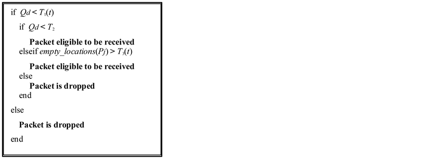
Figure 2. Buffer-management scheme.
destined to monopolizing output ports and reserving some buffer space for underutilized
output ports. The upper bound for the maximum queue length Qmax is regulated
by the dynamic threshold T1(t), while the amount of buffer space reserved
in logical partitions P1, P2, P3,
 , Pn is given by the dynamic threshold T3(t).
The static threshold T2 determines which output ports have access to
the reserved buffer space. The buffer-management scheme can provide quality-of-service
(QoS) to various loss-sensitive traffic classes by using different thresholds values
for different traffic classes. Threshold’s constants should be set to reduce the
probability that high priority packets are dropped. A way to implement priority
control is that traffic classes with high priority see a less restrictive maximum
queue length Qmax and less buffer space is reserved in logical partitions
P1, P2, P3,
, Pn is given by the dynamic threshold T3(t).
The static threshold T2 determines which output ports have access to
the reserved buffer space. The buffer-management scheme can provide quality-of-service
(QoS) to various loss-sensitive traffic classes by using different thresholds values
for different traffic classes. Threshold’s constants should be set to reduce the
probability that high priority packets are dropped. A way to implement priority
control is that traffic classes with high priority see a less restrictive maximum
queue length Qmax and less buffer space is reserved in logical partitions
P1, P2, P3,
 , Pn. Thus, high-priority traffic classes should
have a larger threshold T1(t) value and smaller threshold T3(t)
value compared to low-priority traffic classes. We write this requirement (Equation
(4)) in terms of the tunable constants as follow:
, Pn. Thus, high-priority traffic classes should
have a larger threshold T1(t) value and smaller threshold T3(t)
value compared to low-priority traffic classes. We write this requirement (Equation
(4)) in terms of the tunable constants as follow:
 (4)
(4)
5. Performance Results and Discussion
5.1. Simulation Setup
Bursty traffic is generated using a two state ON-OFF model [1] to evaluate the performance of the SW packet switch. Each input line is connected to an independent bursty source that alternates between active and idle periods of geometrically distributed duration. During an active period, packets arrive continuously in consecutive switch cycles to the input line of the switch. There is at least one packet in an active period. For the duration of an idle period, there are consecutive empty time slots due to the absence of traffic.
The measurements of interest to evaluate the performance of the SW packet switch with the proposed buffer-management scheme are average throughput and average memory utilization. Depending on the offered load, a maximum of 64 × 105 packets were generated. The system considered is a 32 × 32 SW packet switch with a total buffer space of 1024 memory locations. The memory configuration implemented is m = 64 & n = 16, where m is the number of memory modules and n the capacity of each memory or number of logical partitions. All memory modules operate at the line speed R, that is, at most one packet can be written and one packet can be read to/from any memory module during a switch cycle.
5.2. Comparison of Schemes
In Figure 3, proposed buffer-management scheme has a much higher throughput than a previous buffer-management scheme [1] at high loads (>70%) with varying burstiness (6 & 8 packets).
Here, any output queue can extend up to half of the remaining buffer space (α = 0.5) and buffer space is reserved for output ports with queue length Q < n (β = 1 & γ = 0). The proposed algorithm needs to know the length of N output queues, which increases linearly with the switch size N. Thus, the proposed buffer management scheme has O(N) complexity (the same as [1] ).
5.3. One Dimensional Variation
We vary constant α in Figure 4 (and consequentially threshold T1(t)) and set the other two constants fixed at β = 1 and γ = 0.
Figure 4 shows that throughput performance decreases for very small values of the constant α (<0.1). The dynamic threshold T1(t) strongly limits the maximum queue length allowed to output ports for small values of constant α. Thus, many packets destined to active output ports are dropped, even when there is available buffer space, decreasing the throughput performance.
Now we consider varying the constant γ and consequentially the dynamic threshold T3(t). We use fixed values of α = 0.5 and β = 1. For negative values of the constant γ, the buffer-management scheme reserves less buffer space for lightly-loaded output ports. A reduced amount of reserved memory locations in logical partitions causes higher memory utilization as shown in Figure 5. However, this can also lead to inefficient use of the total buffer space and a consequent reduction of the switch performance. On the other hand, for large positive values of the constant γ, many more memory locations are reserved in logical partitions. As a result, the memory utilization decreases as constant γ is larger as shown in Figure 5.
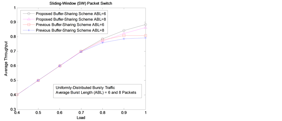
Figure 3. Average throughput comparison between the two SW buffer-management schemes.
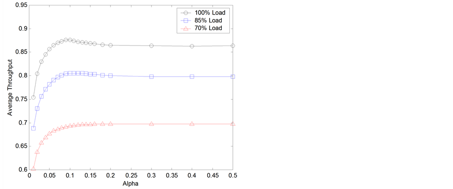
Figure 4. Average throughput varying constant α.
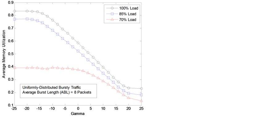
Figure 5. Average memory utilization varying constant γ.
The interaction of the constant β with the other two constants is complex (Figure 6). We should have a value of the static threshold
T2 around the number of logical partitions n or the buffer per port
 to obtain a good performance of the buffer-management scheme. In which,
 is the total buffer space and N is the switch size.
Figure 6 shows memory utilization versus β, T2(β) is a static threshold which doesn’t easily adjust to changes because of its static nature. For small β values it allows underutilized outputs queues to receive packets which increases the memory utilization but as β values increases the heavily loaded outputs queues take more and more of the buffer resources which decreases the overall memory utilization (specially at high loads). After β = 2, T2(β) losses control of the buffer sharing and the other two dynamic threshold basically handle the sharing of the buffer resources. In conclusion static T2(β) is difficult to adjust to change the degree of sharing on the proposed buffer-management scheme, that’s why in Figure 7 only dynamic thresholds T1(t, α), and T3(t, γ) were used to have QoS for two traffic classes.
5.4. Quality of Service
In the simulation experiment in Figure 7, we have two priority classes where half of the incoming packets belong to the high priority class. Using the reference values in (B), we apply a different set of constants for the two
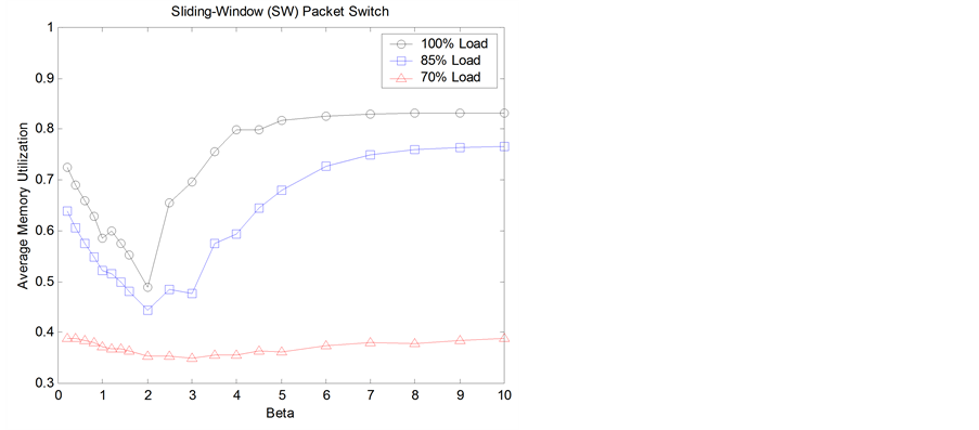
Figure 6. Average memory utilization varying β.
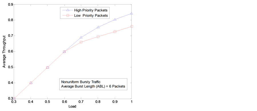
Figure 7. Average throughput of two traffic classes.
priority classes {α, β, γ}. We have {0.5, 1.0, −2.0} and {0.4, 1.0, 2.0} for highand low-priority packets respectively. As shown in Figure 7, throughput is much better for the high-priority class compared to that of the low-priority class. Furthermore, it is evident from Figure 7 that the throughput performance of high-priority packets improves at the expense of decrease in the throughput performance of low-priority packets.
In this section, we address the important issue of QoS in the SW packet switch. The proposed buffer-management scheme can provide QoS by adjusting values for constants α and γ. We should have larger values for the constant α and smaller values for the constant γ for high-priority packets compared to that for low-priority packets.
6. Conclusion
The sliding-window (SW) packet switch is a novel architecture in which the large single memory of the shared-memory switch is replaced by parallel memory modules that can be accessed by all switch ports. The sharing of the buffer space by the output ports has to be regulated by a sharing policy to obtain the optimal switch performance. In this paper, we presented an efficient buffer-management scheme that regulates buffer resources at the global and local level. This scheme utilizes three thresholds to efficiently allocate the buffer resources among the output ports. The simulation results showed a better performance of our buffer-management scheme when applied to the sliding-window packet switch, under identical conditions of switch size, memory size, data traffic, and parallel operation. We also studied the tuning of the buffer-sharing parameters to understand the effect on the performance of the SW packet switch. Finally, we showed how the proposed buffermanagement scheme provided quality-of-service (QoS) for two priority classes.
References
- Kumar, S. (2003) The Sliding-Window Packet Switch: A New Class of Packet Switch Architecture with Plural Memory Modules and Decentralized Control. IEEE Journal on Selected Areas in Communications, 21, 656-673. http://dx.doi.org/10.1109/JSAC.2003.810513
- Choudhury, A.K. and Hahne, E.L.
(1998) Dynamic Queue Length Thresholds for Shared-Memory Packet Switches. IEEE/ACM
Transactions of Networking, 6, 130-140.
http://dx.doi.org/10.1109/90.664262 - Kumar, S., Munoz, A. and Doganer, T. (2004) Performance Comparison of Memory-Sharing Schemes for Internet Switching Architecture. Proceedings of the International Conference on Networking.
- Kamoun, F. and Kleinrock, L. (1980) Analysis of Shared Finite Storage in a Computer Network Node Environment under General Traffic Conditions. IEEE Transactions Communications, 28, 992-1003. http://dx.doi.org/10.1109/TCOM.1980.1094756
- Arpaci, M. and Copeland, J.A. (2000) Buffer Management for Shared-Memory ATM Switches. IEEE Communications Surveys & Tutorials, 3, 2-10. http://dx.doi.org/10.1109/COMST.2000.5340716
- Thareja, A.K. and Agarwala, A.K. (1984) On the Design of Optimal Policy for Sharing Finite Buffers. IEEE Transactions Communications, 32, 737-740. http://dx.doi.org/10.1109/TCOM.1984.1096120
- Munoz, A. and Cantrell, C.D. (2009) Memory-Configuration and Memory-Bandwidth in the Sliding-Window (SW) Switch Architecture. 52nd IEEE International Midwest Symposium on Circuits and Systems, Cancun, 2-5 August 2009, 288-291.
- Yamanaka, K., et al. (1997) Scalable Shared-Buffering
ATM Switch with a Versatile Searchable Queue. IEEE Journal on Selected Areas in
Communications, 15, 773-784.
http://dx.doi.org/10.1109/49.594840 -
Kumar, S. and Munoz, A. (2005) Performance Comparison of Switch Architectures with
Parallel Memory Modules. IEEE Communications Letters, 9, 1015-1017.
http://dx.doi.org/10.1109/LCOMM.2005.11021