Journal of Intelligent Learning Systems and Applications
Vol. 5 No. 1 (2013) , Article ID: 27940 , 9 pages DOI:10.4236/jilsa.2013.51006
Hybrid Methodology for Structural Health Monitoring Based on Immune Algorithms and Symbolic Time Series Analysis
![]()
Department of System Design Engineering, Keio University, Yokohama, Japan.
Email: lrs0809@gmail.com, mita@sd.keio.ac.jp, zhoujin5120@gmail.com
Received October 17th, 2012; revised November 28th, 2012; accepted December 4th, 2012
Keywords: Structural Health Monitoring; Adaptive Immune Clonal Selection Algorithm; Symbolic Time Series Analysis; Real-Valued Negative Selection; Building Structures
ABSTRACT
This hybrid methodology for structural health monitoring (SHM) is based on immune algorithms (IAs) and symbolic time series analysis (STSA). Real-valued negative selection (RNS) is used to detect damage detection and adaptive immune clonal selection algorithm (AICSA) is used to localize and quantify the damage. Data symbolization by using STSA alleviates the effects of harmful noise in raw acceleration data. This paper explains the mathematical basis of STSA and the procedure of the hybrid methodology. It also describes the results of an simulation experiment on a five-story shear frame structure that indicated the hybrid strategy can efficiently and precisely detect, localize and quantify damage to civil engineering structures in the presence of measurement noise.
1. Introduction
Structural health monitoring (SHM) is a vast, interdisciplinary research field whose literature spans several decades. The focus of SHM research is the detection, localization, and quantification of damage in a variety of structures. Broadly speaking, SHM techniques for detecting, localizing, and quantifying damage rely on measuring the structural response to ambient vibrations or forced excitations. Ambient vibrations can be caused by earthquakes, wind, or passing vehicles, and forced vibrations can be delivered by hydraulic or piezoelectric shakers. SHM techniques infer the existence, location and severity of damage by detecting differences in local or global structural responses before and after the damage occurs.
Some success has been achieved with various heuristic optimization algorithms. The annealing algorithm (SA) and genetic algorithm (GA) methods have been used to accurately describe the dynamic behavior of structures [1]. Cunha & Smith used GAs to identify the elastic constants of composite materials [2]. Particle swarm optimization (PSO) has been used to estimate the severity of damage and identify the parameters of shear frame building structures [3]. An improved clonal selection algorithm (CSA), called adaptive immune CSA (AICSA), has been used for structural damage localization and quantification [4,5]. Moreover, recently, a novel pattern identification technique, called symbolic time series analysis (STSA), was developed. The core concept of STSA is the identification of statistical patterns from symbol sequences generated by coarse-graining of time series data. STSA for anomaly detection in complex systems [6] has the potential to deal with noise. Several case studies [7-9] have shown that STSA is more effective at anomaly detection than pattern recognition techniques such as principal component analysis and neural networks. STSA has also been used for fault detection in electromechanical systems, e.g., three-phase induction motors [10].
In this paper, we propose a hybrid methodology combining immune algorithms (real valued negative selection (RNS) and AICSA) and symbolic time series analysis (STSA) for detection, localization and quantification of damage to structural systems. In this methodology, RNS detects damage, and AICSA localizes and quantifies it by minimizing the Euclidean distance between the state sequence histogram (SSH) that STSA gets by transforming the raw acceleration data. We mathematically show that STSA improves noise immunity, and our experimental results show that this hybrid strategy can efficiently and precisely detect, localize and quantify damage to civil engineering structures in the presence of measurement noise.
2. Immune Algorithms and STSA
2.1. Real-Valued Negative Selection and Adaptive Immune Clonal Selection Algorithm
The negative selection (NS) algorithm [11] was inspired by observation of the activity of the human immune system, in particular, the selection process that takes place inside the thymus. In this process, T-cells that recognize the body’s own cells (self cells) are eliminated; this guarantees that the remaining T-cells will recognize only foreign molecules. Gonzalez et al. [12] proposed a new negative selection algorithm that uses a real-valued representation of the self/non-self space. RNS tries to alleviate some of the drawbacks of NS while using the higherlevel-of-representation real space to speed up the detector generation process. Refer to [13] for the detailed procedure of RNS for damage detection.
Inspired by the clonal selection principle (CSP), the clonal selection algorithm (CSA) has been used to deal with optimization problems, thanks its superior search capability compared with classical optimization techniques [14]. CSP explains how an immune response is mounted when a non-self antigenic pattern is recognized by B cells. In natural immune systems, only the antibodies that can recognize the intruding antigens are selected to proliferate by cloning [15]. Hence, the main idea of CSA is that those cells (antibodies) capable of recognizing the non-self cells (antigens) will proliferate. Although CSA has great advantages over GA, it is still difficult to solve complex problems with it. In order to solve complex problems, AICSA embodies three strategies: secondary response, adaptive mutation regulation, and vaccination to speed up CSA’s convergence and ability to find the global optimum. For more information about AICSA, please refer to [16].
2.2. Symbolic Time Series Analysis
It may be appropriate to say that, while classical data analysis focuses on individuals, symbolic data analysis deals with concepts, a less specific type of information. The original time series signals are converted into sequences of discrete symbols, and the statistical features of the symbols can be used to describe the dynamic statuses of a system.
Consider a structural system![]() . The raw acceleration data can be recorded by using sensors. A section of this data, denoted as
. The raw acceleration data can be recorded by using sensors. A section of this data, denoted as , can be obtained by sliding a rectangular window of length
 ![]() along the time series of the raw acceleration data. The first step is to transform the raw acceleration data into a binary symbol series
along the time series of the raw acceleration data. The first step is to transform the raw acceleration data into a binary symbol series .
.  equals “0” or “1” by setting a partition line. After that, we select an integer
  (word length) and define the symbolic state at time
  as the vector
 ![]() containing the subsequent
containing the subsequent  output symbols, namely,
 (1)
(1)
![]() defines a state series
defines a state series . A binary coded
 ![]() should be transformed into the decimal domain, and note that
should be transformed into the decimal domain, and note that ![]() can take
can take  possible values (called “states”), which can be listed as a finite set
 . We can then derive the statistics of the symbolic state, i.e., compute the vector of the observed state frequencies
 , where di (integer
 ) is the number of occurrences of
 . Also, since there are
  states in the state series in total,
  can be normalized as
 . The histogram of
 ![]() and
and  is called the state sequence histogram (SSH).
3. Proposed Method
3.1. Introduction
In our methodology, the self (non-self) element is an SSH gotten by STSA from raw acceleration data from a healthy (damaged) structure. The detector is represented as a redistribution of the states of self elements.
We introduce an index, the relative state sequence histogram error (RSSHe), to measure the distance between two histograms:

 (2)
(2)
where  is the frequency of state
  in
in  or
or .
.
3.2. Procedure
Our methodology has two stages: damage detection using RNS and damage localization and quantification using AICSA. The procedure is as follows (see Figure 1):
Stage 1: Damage detection.
1) Training phase a) To create a subseries of raw acceleration data, a rectangular window of length ![]() is chosen and slid along the raw acceleration data series (length L). A set of subseries numbering
is chosen and slid along the raw acceleration data series (length L). A set of subseries numbering  is created in this way. STSA (Section 2.1) is applied to each sub-series

Figure 1. Procedure of IA and STSA for structural health monitoring.
to create a corresponding 
 .
.
b) To create the self set, the distances  between the jth SSH and all previous
  in the self set is calculated. If one of the distances is less than the predefined self radius
![]() , the jth
, the jth  is discarded. Otherwise, it is stored in the self set as a new self element. This procedure is repeated until the predefined criteria is reached.
c) RNS is applied to the self set to generate detectors.
2) Detection phase a) New raw acceleration data of a structure is symbolized into a corresponding  by using the same method as in step a) of the training phase.
b) When matching  with the detectors generated in the training phase, if any detectors are activated (the distance between them is less than a certain value), a signal indicating the occurrence of the abnormal structural state will be given.
Stage 2: Damage localization and quantification.
In the research field of structural parameter identification, the time response of the system is usually compared with that of a parameterized model using a norm or some performance criterion to give us a measure of how well the model explains the system.
Suppose that damage to a structure has been detected by the above procedure. Moreover suppose that there is a parameterized model able to capture the behavior of the physical system, and this model depends on a set of n parameters, i.e., . Given a candidate parameter value
 ![]() and a guess
and a guess  of the initial state,
  , the value of the parameterized model, i.e., the identified system at the ith discrete time step, can be obtained. Hence, the problem of system identification boils down to finding a set of parameters that minimize the prediction error between the system output
 , which is the measured data, and the model output
  which is calculated at each time instant
 .
.
Usually, our interest would lie in minimizing the predefined error norm of the time series outputs, e.g., the following mean square error (MSE) function,
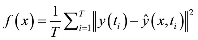 (3)
(3)
where  represents the Euclidean norm of vectors. Formally, the optimization problem requires one to find a set of
 ![]() parameters
parameters  so that a certain quality criterion is satisfied, namely, that the error norm
  is minimized. The parameters of the model are taken to be equivalent to the parameters of the structure.
In our methodology, instead of comparing raw acceleration data directly, the Euclidean distance of SSHs from the structure and model is used as a measure of the distance between the system output  and model output
 .
.
3.3. Generation of Detectors
If window length is ![]() and word length is
and word length is , the number of states in
  is
is  and the minimum changeable unit is
 , then the total number of possible distributions
  of SSH is equal to one classic combination problem, which is ‘put
  same balls in
  different boxes, and the combinatorial number is:
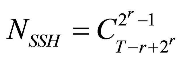 . Supposing that the
  can capture the dynamic features of a structure, the normal state of the structure is represented by
  (self), the damage to that structure can be expressed by other distributions of states in the
  (non-self). Instead of randomly generating candidate detectors (which may result in creating an impossible distribution of states in the
 ), a novel procedure to create candidate detectors on the basis of self elements is proposed. The procedure is described below (
 is the number of self elements).
1) Redistribution: Randomly choose n (integer
 ) states from
 . Randomly changing the frequency values of the
 ![]() chosen states and keep their sum unchanged. Note that the minimum unit of change is
chosen states and keep their sum unchanged. Note that the minimum unit of change is . The newly created
by this procedure is used as the candidate detector.
2) Self recognition: Calculate the distance between candidate detector and all self elements. If the minimum distance  (
(![]() is self radius), delete it. If not, keep it for the next step.
is self radius), delete it. If not, keep it for the next step.
3) Recognition of existing detectors: Calculate the distance between the candidate detector and the existing detectors. If the minimum distance  (
( is the radius of existing detectors;
 ![]() is the overlap rate, defined in 3.4), delete it. If not, store it as a new detector. Set
is the overlap rate, defined in 3.4), delete it. If not, store it as a new detector. Set  as the radius of the new detector.
Repeat Steps (1) - (3) until the predefined stopping criterion is reached.
3.4. Noise Immunity
Usually the raw acceleration data is chosen as input, and the Euclidean distance of raw acceleration data is used as the damage index or objective function; the problem is that the possible number of representations of raw aceleration data is infinite for any Euclidean distance. In other words, the raw acceleration data is easily affected by noise. STSA is a coarse graining process that is robust against measurement noise. It is expected that small changes in time series data do not affect the symbolized data. Therefore, it can be assumed that a certain band of states represents similar dynamic status of the dynamic structural system, and instead of having an infinite number of representations of the Euclidean distance in the case of using raw acceleration data as input, the  representation is finite.
Taking a SDOF (single degree of freedom) system as an example, the dynamic equation can be represented as:
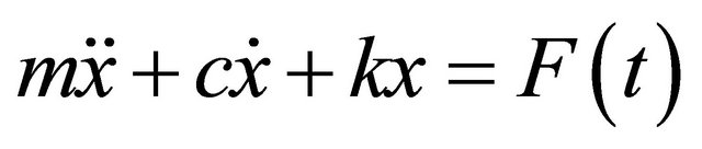 (4)
(4)
where![]() ,
, ![]() , and
, and  are respectively the mass, damping ratio, and stiffness of the system, F is the force linked to the ground acceleration. By dividing both sides by the mass
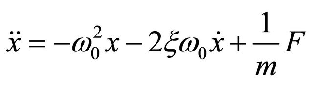
![]() , the equation of motion becomes
, the equation of motion becomes
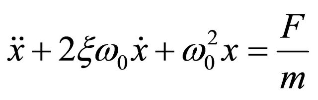 (5)
(5)
where
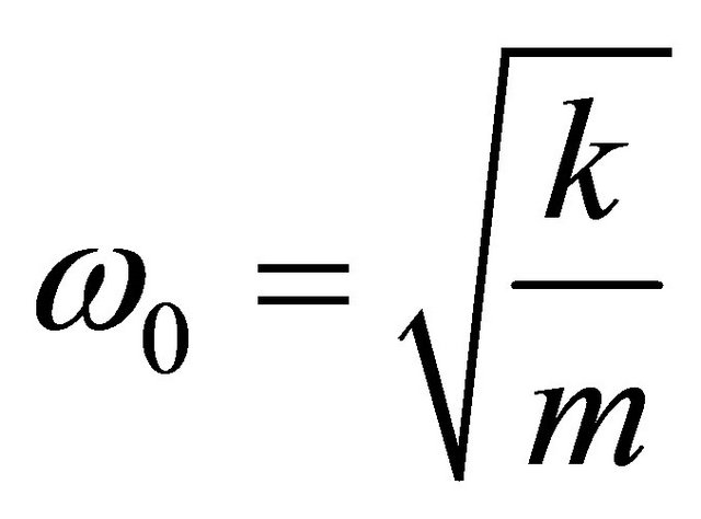 : undamped natural frequency of the oscillator
 : damping ratio The value
 (6)
(6)
is called the critical damping.
Acceleration  is:
is:
 (7)
(7)
At time ,
,  can be obtained as
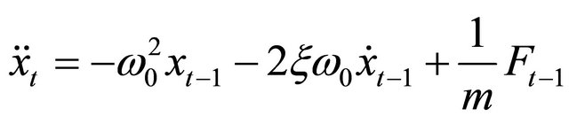 (8)
(8)
Since the window length is ![]() and word length is
and word length is , all the raw acceleration data in the window is
  . The mean value of
  is:
is:
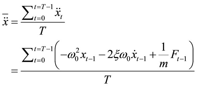 (9)
(9)
This mean value of  is for the noise-free case. In case of raw acceleration data polluted by noise, the acceleration data at time
  is
is
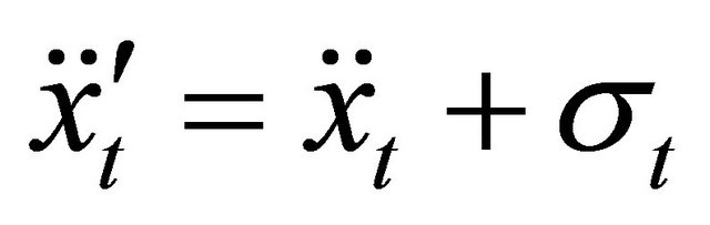 (10)
(10)
where  is the value of noise at time
 . The partition line (the mean value of
  ) is:
) is:
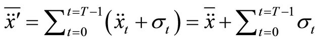 (11)
(11)
For a sufficiently long window length ![]() and word length
and word length ,
,  , which means that noise will not affect the partition line.
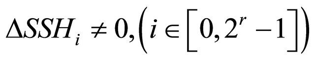
A random sample of SSH is defined as . From Equation (2), any other
  (i.e.,
 ) will be some distance away from
 .
.
 (12)
(12)
where
 and
and  (13)
(13)
where  and
and  is an even number.
From reference [18], since the minimum unit of change in  is
is  and the dimension of
  is
is
 , there is a possibility that not only one but many different
  will have the same
  as
as . This possibility occurs when Equation (13) is satisfied.
The minimum number of  s that have the same
  as
as  occurs when the difference between
  and
and  is only one minimum unit; in that case,
  , the minimum number is:
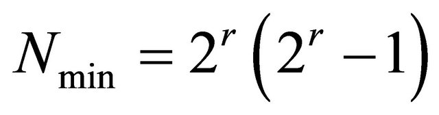 . If there are two different minimum units between
  and
and ,
, ![]() equals 4, 6 or 8.
equals 4, 6 or 8.
 , where
  is the number of different units between
  and
and . The number of different values of ε is
 . For every certain value of ε can be called as a representative band, then the number of representative band is
 . Also, we can see that for a certain combination of
 , when α is the number of elements for which
 , the possible combinatorial
number is . For example, when
  and
and ![]() is the minimum 2, the combinatorial number is 130816, which is a big number, and we should note this is only the minimum one. The conclusion is that STSA has very good fault tolerance.
is the minimum 2, the combinatorial number is 130816, which is a big number, and we should note this is only the minimum one. The conclusion is that STSA has very good fault tolerance.
In addition, since the total number of units in  is
is ,
, . For each representative band
![]() , there will be many representations of
, there will be many representations of ; in other words, a small change in the raw acceleration data (say, due to noise) will not affect the
  between
  and
and .
.
3.5. Indexes Used in the Performance Evaluation
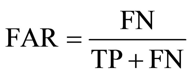
Two indexes are used to evaluate the classification accuracy: the detection rate (DR) and the false alarm rate (FAR). DR is the ratio of correctly classified negative elements to the total negative elements, and the FAR is the ratio of incorrectly classified positive elements to the total negative elements. Four values are needed to calculate DR and FAR: the number of true positives (TP, positive elements identified as positive), true negatives (TN, negative elements identified as negative), false positives (FP, negative elements identified as positive), and false negatives (FN, positive elements identified as negative). DR and FAR are calculated as
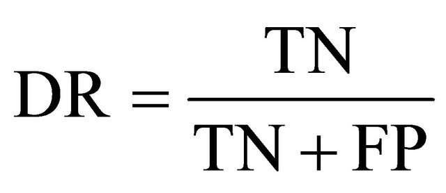 (14)
(14)
 (15)
(15)
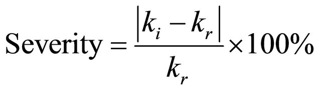
In the damage localization and quantification stage, the severity of damage is defined as
 (16)
(16)
where ![]() and
and  are the identified stiffness and real stiffness of the
  th story, respectively.
4. Numerical Simulation
4.1. Description of Model
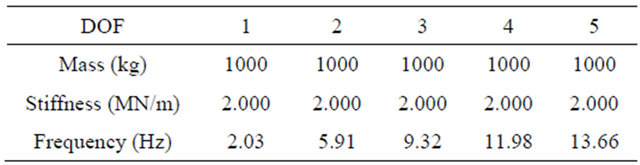
For simplicity and generality, we used a five-story shear frame structure as a representative case to verify the performance of our methodology, and we modeled it as a five degree-of-freedom lumped mass system (Figure 2). Table 1 lists the structural and modal parameters of the structure.
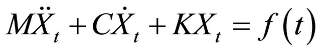
The dynamic equation is [17]:
 (17)
(17)
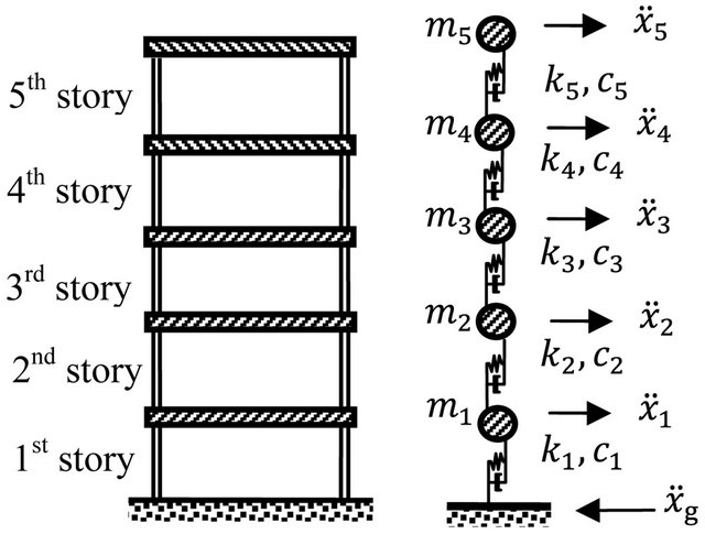
Figure 2. 5-DOF shear frame structure.
Table 1. Structural and modal parameters of the structure.
where ,
,  , and
, and  are respectively the mass matrix, damping matrix, and stiffness matrix.
  is the force vector linked to the ground acceleration.
 ,
,  , and
, and  are respectively relative acceleration, velocity, and displacement response. The sampling frequency was 100 Hz. In the simulation, the input signal was Gaussian white noise (Figure 3). To test the noise immunity of our method, noise at levels of 5% and 10% was added to the raw acceleration data.
4.2. Results of Damage Detection
The training data sets that were to generate detectors were acceleration time histories from the top story of the healthy shear structure under ground motion following a pattern of randomly generated Gaussian white noise. In the test phase, the test data sets (self and non-self) were obtained from the top story of the healthy and damaged shear structure under ground motion following another pattern of randomly generated Gaussian white noise. The sampling frequency was 100 Hz, and all time histories were normalized.
As is shown in [18], the word length and window length will greatly affect the performance of the methodology. Larger word and window lengths yield better performance. The reason is that, a longer word or window can symbolize the raw acceleration data much more accurately than a shorter one. As the word length and window length increase, much more dynamic information about the system is captured, and the representation space of the problem becomes more accurate. In the simulation, the word length was set as 9 and window length was set as 3.0E+03.
Several tests were performed by simulating stiffness reductions occurring in different locations and to different degrees. The simulated cases included stiffness re-
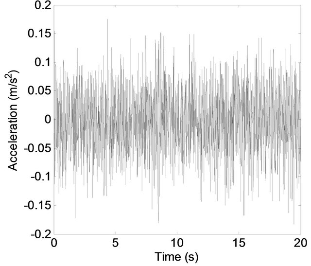
Figure 3. Example input signal (Gaussian white noise).
ductions on a single story (2nd story or 4th story) and on two stories (2nd story and 4th story). The degree of stiffness reduction was 10% or 20%. Table 2 lists the most pertinent results, and Figure 4 compares the DR and FAR values of the different damage cases.
The results show that, by employing our methodology, perfect results can be obtained for the noise-free case, DR is 100% and FAR is 0%, which means all the damage can be detected and no SSH from the healthy structure is misclassified. For the noise polluted cases as well, a high DR and low FAR can be obtained no matter the location or degree of stiffness reduction. Even as the noise level increases and the detection rate decreases, the extent of misclassification remains very small. This means that noise is not problematic in our methodology. Indeed, the good results probably reflect the fact that the RSSHe is much more sensitive to changes in the structure itself than to the environment.
5. Numerical Simulation of Damage Localization and Quantification
5.1. Description of Procedure
In this simulation, the system to be identified was the same five-story shear frame structure as stated before; the mass distribution and damping parameters were assumed to be known, and the stiffness of each story was set as the objective parameters that needed to be identified. First, the parameters of the healthy structure were identified as a reference. AICSA was performed when the abnormal SSH of the damaged structure was detected. The abnormal SSH was the output of the damaged structure. The input ground acceleration data corresponding to the abnormal SSH was used as the input of the candidate model, and the output of the candidate model was symbolized using the procedure in Section 2.2. The Euclidean distance of system and candidate SSHs was used as the objective function to be minimized. After the parameters of the damaged structure were identified, the severity (Equation (6)) showing the location and degree of the
Table 2. DR and FAR of different damage cases.
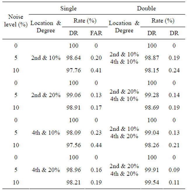
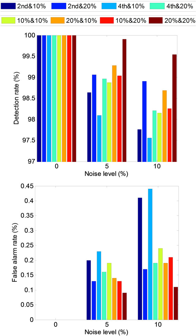
Figure 4. DR and FAR for damage detection.
damage was calculated.
5.2. Identification Results for Healthy and Damaged Structures
The input signal was Gaussian white noise, as in the previous simulation. The window and word lengths were the same as before, and the full output of the structure was used. Table 3 lists the identified stiffness of each story of the healthy and damaged structures. The damage cases are the same as those in the damage detection stage. Severity of damage was calculated for each damage case using the results in Table 3, and Figures 5, 6 and 7 plot the severity for the noise-free, 5% noise and 10% noise cases, respectively.
Table 3. Estimated parameters for healthy and damaged models with a word length of 9 and window length of 3000.
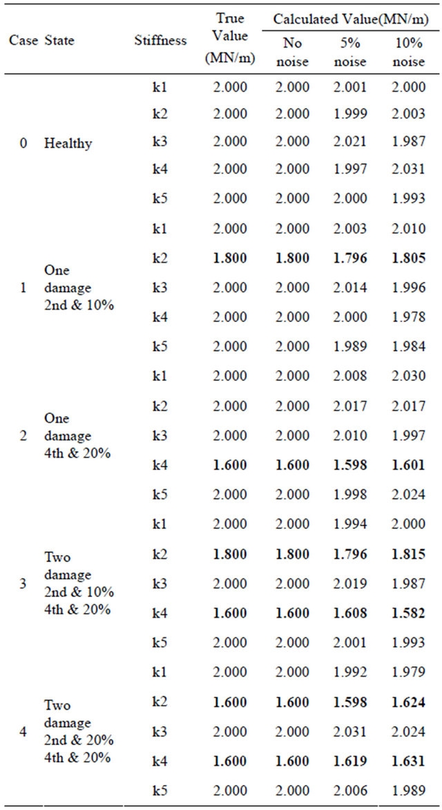
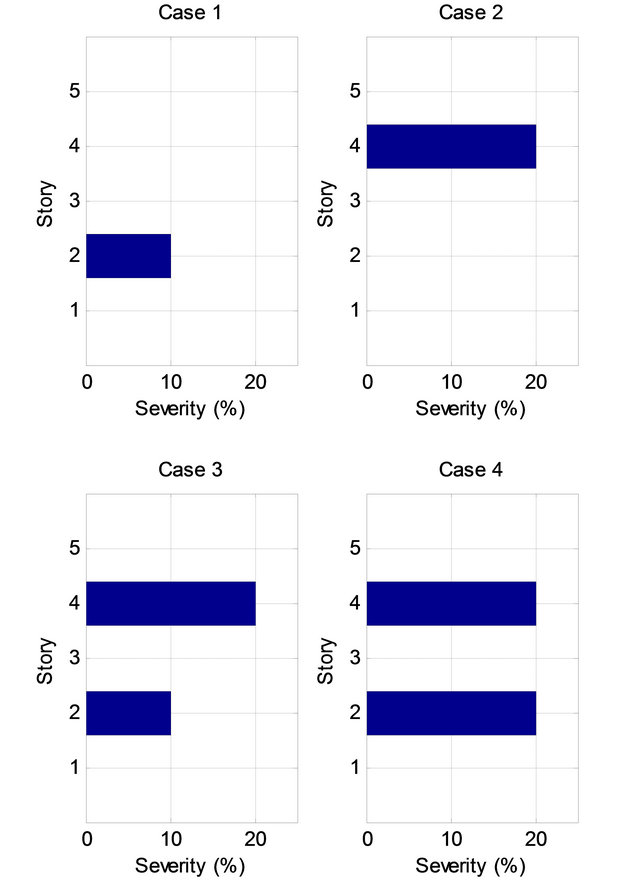
Figure 5. Identification results for noise-free case.
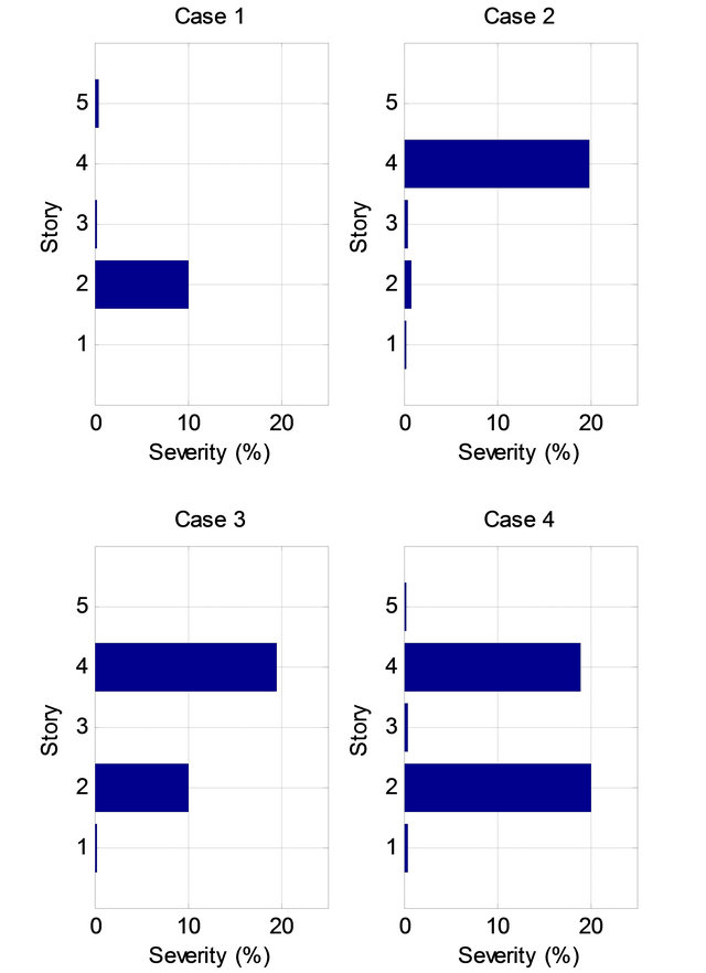
Figure 6. Identification results for 5% noise case.
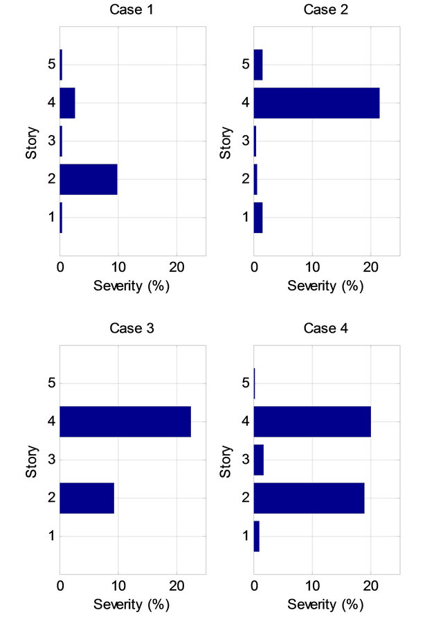
Figure 7. Identification results for 10% noise case.
The results show that, AICSA combining STSA can identify the parameters of a structure accurately regardless of whether the structure is healthy or damaged. Even error of severities of each story increase slightly as the noise level of the raw acceleration increase, the location and severity of the damage can be identified distinctly.
6. Conclusion
We proposed a hybrid methodology based on immune algorithms (IAs) and symbolic time series analysis (STSA) for structural health monitoring (SHM). In this methodology, RNS is used detect damage, and AICSA is used to localize and quantify the damage to the structure. Data symbolization by using STSA alleviates the effects of noise in the raw acceleration data. We explained the mathematical basis of STSA and described a simulation experiment on a five-story shear frame structure. The results showed that this hybrid methodology can efficiently and precisely detect, localize and quantify damage to civil engineering structures in the presence of measurement noise.
7. Acknowledgements
This work was supported in part by a Grant-in-Aid No. 22310103 (PI: A. Mita) and Grant-in-Aid of the Global Center of Excellence Program for the “Center for Education and Research of Symbiotic, Safe and Secure System Design” from the Ministry of Education, Culture, Sport, Science and Technology of Japan.
REFERENCES
- R. I. Levin and N. A. J. Lieven, “Dynamic Finite Element Model Updating Using Simulated Annealing and Genetic Algorithms,” Mechanical System and Signal Process, Vol. 12, No. 1, 1998, pp. 91-120. doi:10.1006/mssp.1996.0136
- K. Cunha and V. V. Smith, “A Determination of the Solar Photospheric Boron Abundance,” Astrophysical Journal, Vol. 512, No. 2, 1999, pp. 1006-1013. doi:10.1086/306796
- S. T. Xue, H. S. Tang and J. Zhou, “Identification of Structural Systems Using Particle Swarm Optimization,” Journal of Asian Architecture and Building Engineering, Vol. 8, No. 2, 2009, pp. 517-524. doi:10.3130/jaabe.8.517
- R. Li and A. Mita, “Structural Damage Identification Using Adaptive Immune Clonal Selection Algorithm and Acceleration Data,” SPIE Smart Structures/NDE2011, San Diego, 6-10 March, 2011, 79815A.
- R. Li and A. Mita, “Hybrid Immune Algorithm for Structural Health Monitoring Using Acceleration Data,” 8th International Workshop on Structural Health Monitoring, Stanford University, 13-15 September 2011, pp. 1095-1102.
- A. Ray, “Symbolic Dynamic Analysis of Complex Systems for Anomaly Detection,” Signal Processing, Vol. 84, No. 7, 2004, pp. 1115-1130. doi:10.1016/j.sigpro.2004.03.011
- S. Chin, A. Ray and V. Rajagopalan, “Symbolic Time Series Analysis for Anomaly Detection: A Comparative Evaluation,” Signal Processing, Vol. 85, No. 9, 2005, pp. 1859-1868. doi:10.1016/j.sigpro.2005.03.014
- A. Khatkhate, A. Ray, S. Chin, V. Rajagopalan and E. Keller, “Detection of Fatigue Crack Anomaly: A Symbolic Dynamic Approach,” Proceedings of American Control Conference, Boston, 30 June-2 July 2004; pp. 3741-3746.
- D. Tolani, M. Yasar, A. Ray and V. Yang, “Anomaly Detection in Aircraft Gas Turbine Engines,” AIAA Journal of Aerospace Computing Information, and Communication, Vol. 3, No. 2, 2006, pp. 44-51. doi:10.2514/1.15768
- S. Bhatnagar, V. Rajagopalan and A. Ray, “Incipient Fault Detection in Mechanical Power Transmission Systems,” Proceedings of American Control Conference, Portland, 8-10 June 2005, pp. 472-477.
- S. Forrest, A. Perelson, L. Allen and R. Cherukuri, “SelfNonself Discrimination in a Computer’,” Proceedings of IEEE Symposium on Research in Security and Privacy, Los Alamitos, 16-18 May 1994, pp. 202-212.
- F. Gonzalez, D. Dasgupta and R. Kozma, “Combining Negative Selection and Classification Techniques for Anomaly Detection,” Proceedings of the 2002 Congress on Evolutionary Computation CEC2002, 12-17 May Honolulu, pp. 705-710.
- F. A. Gonzalez and D. Dasgupta, “Anomaly Detection Using Real-Valued Negative Selection,” Genetic Programming and Evolvable Machines, Vol. 4, No. 4, 2003, pp. 383-403.
- X. Wang, X. Z. Gao and S. J. Ovaska, “Artificial Immune Optimization Methods and Applications: A Survey,” Proceedings of the IEEE International Conference on Systems, Man and Cybernetics, The Hague, 10-13 October 2004, pp. 3415-3420.
- J. Timmis, P. Andrews, N. Owens and E. Clark, “An Interdisciplinary Perspective on Artificial Immune Systems,” Evolutionary Intelligence, Vol. 1, No. 1, 2008. pp. 5-26. doi:10.1007/s12065-007-0004-2
- L. Zhang, X. R. Meng, W. J. Wu and H. Zhou, “Network Fault Feature Selection Based on Adaptive Immune Clonal Selection Algorithm,” 2009 International Joint Conference on Computational Sciences and Optimization, Sanya, 24-26 April 2009, pp. 969-973. doi:10.1109/CSO.2009.342
- A. Mita, “Structural Dynamics for Health Monitoring,” Sankeisha Co., Ltd, Nagoya, 2003.
- R. S. Li, A. Mita and J. Zhou, “Feasibility Study of Parameter Identification Method Based on Symbolic Time Series Analysis and Adaptive Immune Clonal Selection Algorithm,” Open Journal of Civil Engineering, Vol. 2 No. 4, 2012, pp. 198-205.