Journal of Water Resource and Protection
Vol.5 No.3(2013), Article ID:28906,10 pages DOI:10.4236/jwarp.2013.53030
Leakage Detection in Water Distribution Network Based on a New Heuristic Genetic Algorithm Model
1Civil Engineering College, Ferdowsi University of Mashhad, Mashhad, Iran
2Hydraulic Engineering, Part Mahan Co., Mashhad, Iran
Email: ali_geran@yahoo.com
Received December 1, 2012; revised December 31, 2012; accepted January 8, 2013
Keywords: Calibration; SSEM; Water Distribution; Leak Detection; Genetic Algorithm
ABSTRACT
The leakage control is an important task, because it is associated with some problems such as economic loss, safety concerns, and environmental damages. The pervious methods which have already been devised for leakage detection are not only expensive and time consuming, but also have a low efficient. As a result, the global leakage detection methods such as leak detection based on simulation and calibration of the network have been considered recently. In this research, leak detection based on calibration in two hypothetical and a laboratorial networks is considered. Additionally a novel optimization method called step-by-step elimination method (SSEM) combining with a genetic algorithm (GA) is introduced to calibration and leakage detection in networks. This method step-by-step detects and eliminates the nodes that provide no contribution in leakage among uncertain parameters of calibration of a network. The proposed method initiates with an ordinary calibration for a studied network, follow by elimination of suspicious nodes among adjusted parameters, then, the network is re-calibrated. Finally the process is repeated until the numbers of unknown demands are equal to the desired numbers or the exact leakage locations and values are determined. These investigations illustrate the capability of this method for detecting the locations and sizes of leakages.
1. Introduction
In many towns, the daily water loss is about 40% - 50% of the total daily water consumption [1] which causes economic, environmental and safety costs [2,3]. The low quality of the material using in pipes, design errors, inadequate maintenance, applying the network in a high pressure condition and also random failures are only some of the reasons causing damage within the network [4]. Thus, the occurrence of leakages is unavoidable and the leakage control is an important task. The leak detection methods are generally divided into two main groups. The first one is the local leak detection methods: In this group, water distribution system (WDS) is being divided into several parts and for each part; leakage is searched by using various equipments [5]. Acoustic equipment, mass balance technique, thermography, ground-penetrating radar, tracer gas, and video are the most popular methods. These methods are costly, labor intensive and often limit accuracy and none of them has proven to be completely successful [3,6,7]. The second group is global methods: Network-monitoring system is installed and some information includes nodal pressures and pipe flows are recorded; then the network is analyzed to determine the leaky point [8]. Accurate determination of network parameters is usually associated with some errors that roughness, nodal demands and valve statues are the most difficult ones to determine [5]. Therefore, the simulated model results have some discrepancy with the pressure and flow measurement in networks.
The calibration process consists of adjusting undetermined parameters to obtain the same nodal pressure and pipe flow in model analysis results and measurements [8,9]. Calibration approaches are classified into trial-anderror procedures [10-13], explicit methods [14-17] and implicit models [18-20]. Implicit methods are used widely to formulate an objective function that should be minimized. The objective function is related to the differences between observed and calculated head and flow parameters.
Walski et al. considered the automated calibration accuracy approach for steady flow by using some pressure transducers for a laboratory model. It has been shown that the proposed method is quite suitable and provides good accuracy for determining the friction factor, nodal demand and, valve status [21]. Lingireddy and Ormsbee studied network optimization to define friction factor and demand based on the computer models they tried to confirm the efficiency of artificial calibration method [22]. In their calibration method, friction factor are accomplished by fire flow tests in five groups. In the next step, the nodal demands are estimated using the extended period simulation (EPS) in the same network. Also, they proposed to use the fire flow test and EPS for calculating the friction factor and the nodal demand, respectively [22]. Kang and Lansey performed the demand and roughness calibration upon two networks based on a twostep method [23]. They used the roughness and nodal grouping to limit the uncertain parameters [23]. Cheng and He calibrated the nodal demands based on pressures measurements in Hangzu, China [24]. The unknown parameters in a network are considerably more than the observations; therefore, the calibration procedure should be treated as a problem suffering numerous degrees of freedom. Accordingly, some researchers have focused on the reduction of the freedom degrees applying the nodes and pipe grouping [22-25]. Another way to improve the calibration is increasing the observation numbers via the EPS, analyzing the network during fire flow test and the transient analysis [22-26].
Almandoz et al. and Walski et al. developed another method for indicating the leakages using network hydraulic simulation [27,28]. Wu and Sage followed their work and studied the leak detection in the WDS based on a genetic algorithm optimization and pressures calibration [8]. Fazel and Maghrebi accomplished a research in the network of Golbahar city to detect the leakages via GA. The results confirmed the usefulness of this method for detecting the leakages, however to achieve acceptable results, a large number observations should be performed [29].
The objective of the current paper is detecting the location and magnitude of the leakages of networks. A novel approach is introduced that employ a two-phase analysis. As the first phase, the network are calibrated a number of times with different optimization parameters. The second phase is initiated with establishing two groups of the nodes include “leakage nodes” and “no leakage nodes”. For each calibrating case of Phase 1, the nodes that their calculated demands are sufficient higher than the base demands are located in the leakage nodes. Also, the nodes, which their computed demands are equal or less than the base demands, are placed in the no leakage nodes. Obviously, it is possible that a node in an analysis sets in one group, but in the next analysis is placed in the other ones. After doing this process for all of the calibration cases of Phase 1, the nodes that placed in the no leakage nodes and are never determined as one of the leakage nodes, are eliminated from the unknown demands, and they is fixed as base demands in the next stages. These processes are repeated until the interest results are obtained. The applications of this method for two hypothetical and one experimental networks are shown an amazing improvement of leakage detection than a single genetic algorithm. It should be mentioned that this method can be associated with any optimization method to improve its capability.
2. Methodology
2.1. Calibration Methodology
In a WDS, calibration is used for determination of actual unknown parameters. The adjustable parameters are the friction factor ( ) of the pipe
  (Hazen-Williams factor), the demand multiplayer
  for the node
 at time
  and the valve status
 , for the valve number
  [8]:
[8]:
 (1)
(1)
where is the set of the unknown parameters,
  ,
,  and
and  where
where ,
,  and
and  are the number of the pipe groups, the adjusting valve and the junction groups, respectively. The fitness function that should be minimized is [8]
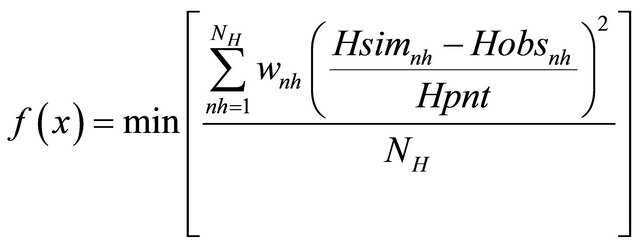 (2)
(2)
Under the conditions of:
 (3)
(3)
where  is the objective function that shows the differences between the measured and simulated values.
 ,
,  and
and  are the measured, calculated and adjusted parameters of each node, respectively and
  is the number of pressure measurement.
  is the total number of the observation nodes and
 is the weight index.
  and
and  show the lower and upper limits for the roughness of the
  pipe, respectively,
  and
and  are the lower and upper limits for the adjusted demand multiplayer of node
 , respectively [8]. The adjusting calibration parameters in this paper are only demands and no grouping is used for reduction of the unknown parameters.
2.2. Optimization Methodology
Genetic algorithm (GA) is used in various fields of sciences and its capability has been proved in finding the optimal points for different problems. This method is an evolutionary based method and potential solutions for a problem is represented as coded strings. A population of these solution strings are kept and subjected to evolutionary operators. Three main operators of GA are selection, cross-over and mutation [30]. In this method, a stochastic search is begun by creating a number of solution strings named “Initial Population” [30] and fitnesses for strings are evaluated using Equation (1). To produce the next generation, strings are randomly chosen from the initial population based on their fitnesses, and then crossover and mutation are operated on the strings. Crossover is responsible for transition the parent’s traits to their child. The mutation randomly changes a string to recover new traits. In the GA, population evolves after a number of generations and can attain the optimal solution. Up to now, many approaches are presented based on general principles of GA. Also, this method is used in the WDS calibration and leakage detection [8,9,21,31]. In the current paper a simple GA joining with is used SSEM for the optimization process.
2.3. Step-by-Step Elimination Method
During a research, when GA was applied to calibrate a small network, it was observed that GA was not able to determine the exact location and value of leakages. By changing the crossover and mutation, different locations and values for leakages were obtained, while there was no certainty in the result authenticity. It was remarkable that in some nodes, no leakages in several analyses were detected. The calibration results, after omitting these nodes, illustrated some other nodes without leakages. The third analysis after elimination of these nodes, could define values and positions of the leakages, precisely. Applying this method for bigger networks is approved the usefulness of the method. This method has presented as a flowchart illustrated in Figure 1.
In this flowchart, t and s are the numbers of analysis in a step, and the number of steps, respectively.  has the lowest value until
  analyses, and
  is nodal fitness of the
 . The tc counts the numbers of analyses without any improvement in the fitness, and
  is the maximum number tc that should end Phase 1. T is the maximum number of Phase 2,
  is the least fitness which is acceptable according to the accuracy of input data for optimization results. The NH shows the numbers of eliminated nodes during each calibration stage, NR is the remaining nodes and
  is the minimum numbers of nods which are calibrated during the final stage.
According to Figure 1, SSEM is divided into two main phases. In phase one which is dealt with optimization using GA, the network is calibrated for finding an
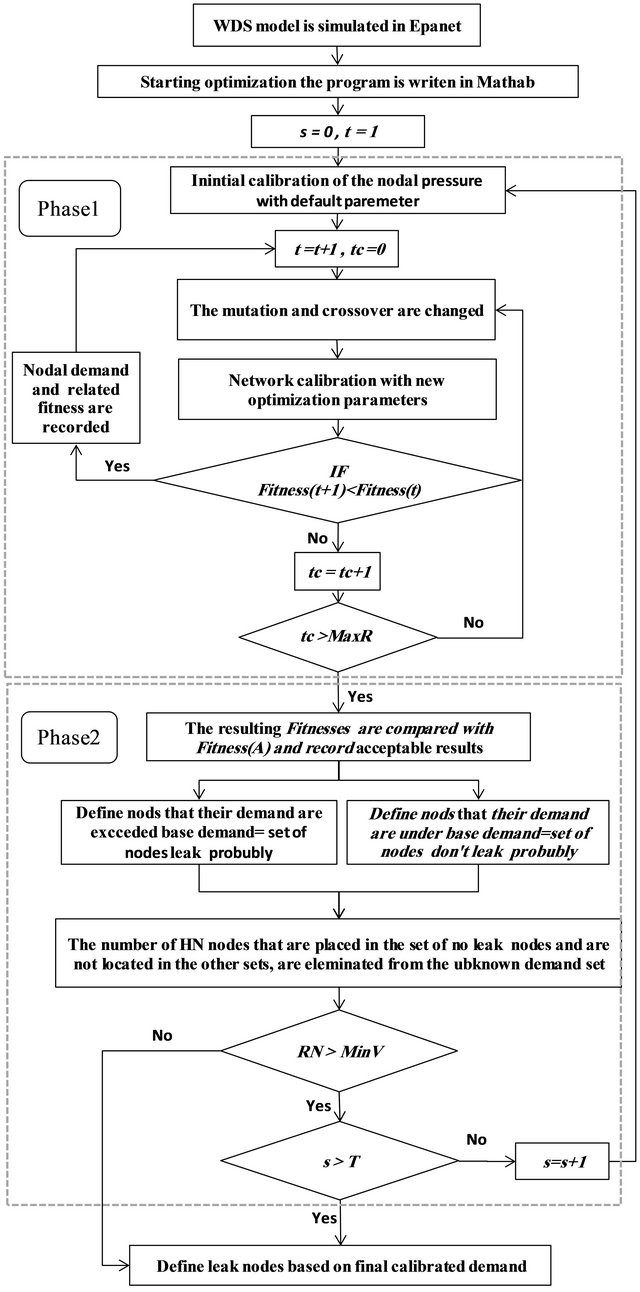
Figure 1. Flowchart of calibration.
unknown demands set with default optimization parameters, then crossover and mutation operators are randomly changed to find a new solution including the demands set and related fitness. If these sets lead to a better fitness, the process will be repeated; otherwise, the next phase will be begun. In Phase 2 the node elimination is performed. Different values of the fitnesses are obtained by using a number of crossover and mutation parameters. They are compared with acceptable fitness. The acceptable fitness is estimated by designers using a trial and error process in accordance with the network dimensions, number of observations and measurement accuracy. The simulated demands set obtained in various network calibrations is compared with the base demands set. The nodes that their consumption are enough higher than their base demands are demands with leakage values in comparison with the base demands are considered as leaky set. On the other hand, the nodes with equal or less demands than the base ones are considered as the nodes with no leak. It should be noted that the base demands are calculated based on the customer consumptions metering. In the final step, the nodes which are located in the second set and also were not being placed in the first set are eliminated from the unknown demand list and the base demands are assigned to these in the next analysis. In this paper, in addition to the usual fitness function , another fitness function which is introduced by Equation (4), is used to check the accuracy of leakage detecting results:
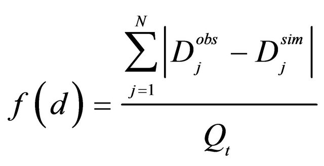 (4)
(4)
where  is the demand fitness, N is the number of network nodes and
  is the actual demand and
  is the simulated demand at node j in the network.
  is the total inflow to the network.
3. Case Studies
Two hypothetical and one laboratorial networks have been used in this investigation. The first network has presented the process of this method. The second network has applied on a bigger network to show the capability of the approach and final network, the laboratorial network, has evaluated the method with the real data.
3.1. Case 1
According to Figure 2 the first network comprises six nodes and nine pipes in two loops. The elevation of the reservoirs 1 and 2 are 100 and 30 meters, respectively.
In the output pipe, a half-open valve with a minor loss coefficient of 10 was embedded. The pipe characteristics and corresponding discharges are given in Table 1. The model is studied under two load conditions. Column 1 of the Table 2 indicates the first load condition that the nodal demands are equal to the base demands (0.2 l/s for each node). Column 2 presents the second condition of

Figure 2. The schematic model of network number 1.
loading with two simultaneous leakages in nodes number 3 and 5. Discharge of 0.5  is added to the base demands of each node. The pressures of the nodes 2 and 4, obtained from the second case of loading condition, are used as the observations.
SSEM is applied to find the leakage among the six unknown demands in the network using two observations. Results have been shown in Table 3. The first stage, including four analyses, has improved the fitness of 0.0189 to 0.0088. The nodes 1, 3, 5 and 6 are introduced as the high demand nodes and the nodes 1, 2, 3, 4 and 5 as the low demand nodes. It should be noted, the high and low demands refer to the demands more than 0.4 and less than 0.2 l/s, respectively.
Since node 2 is not known as a leaky node and it has always been revealed as one of the minimum demand nodes, it is eliminated from the adjusted demand parameters. In the second stage five unknown demands should be adjusted. This will be carried out by calibration of the network in four different cases of crossover and mutation operators. The results reveal that the node numbers 1 and 4 are candidate for elimination in this stage. By eliminating nodes 1, 2 and 4 from the list of suspicious nodes to leakage, searching should be accomplished in the remained nodes of 3, 5 and 6 in the third
Table 1. Pipe Characteristics in the network 1.

Table 2. Demands and pressures in the two load conditions.
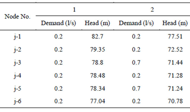
Table 3. The calibration process.
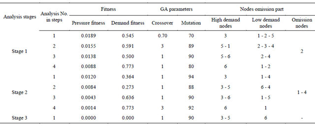
stage. Analysis In the next stage will be led to a fitness value of zero for the pressure. The results in the last analysis indicate a demand of 0.7 l/s in the nodes 3 and 5. Figure 3 shows the changes of the nodal pressure and nodal demands fitnesses obtained in nine consequent analyses. The details of results are presented in the Table 3. In this table, two fitness functions of pressure and demand in a non-dimensional form, calculated based on Equations (2) and (4), respectively, are presented. In this table, the fitnesses of pressures and demands, GA parameters and node sets are presented in a non-dimensional form.
It should be noted that the improvement in the nodal pressure fitness does not necessarily guarantee the amelioration in the nodal demand fitness as well as detection of leakage in the network. From Figure 3, although the pressure fitness after the eighth analysis reduces to a small amount of 0.0014, the demand fitness shows a large amount of deviation in the calibration results. Although the pressure fitness function approaches zero, limitation in the numbers of observations may lead the calibration to incorrect results [21]. Also, since there is not a straight forward way for selecting the crossover and mutation parameters to improve the pressure fitness, it is recommended to calculate the network with different GA parameter values.
3.2. Case 2
Network 2, introduced by Poulakis et al. [32], includes twenty loops, thirty junctions, fifty pipes, and one reservoir. The lengths of horizontal and vertical pipes are 1000 and 2000 meters, respectively. The average height of the roughness for all of the pipes is 0.26 mm and the nodal demand for each node is 50 l/s. The diameters of the pipes are shown in Figure 4.
Poulakis et al. applied the Bayesian probabilistic framework to detect 22.8 l/s of leakage in the node number 26 [32]. Two observational cases including pressure measurements in seven nodes and flow measurements in seven pipes were considered in this research. Some uncertainty with an average of zero in the range of the (−a, a), (−b, b) and (−c, c) were allocated for roughness, demand and measurement, respectively. The analyses were performed in various cases including no error measurement, 5 and 10 percent error in the roughness, 2 and 5 percent error in the nodal demands and finally 2 and 5 percent error in the measurements. The network was analysed separately for all of the observational cases and unknown parameters with different errors. No simultaneous adjustment of the roughness and demand was applied.
Also, they simplified the problem supposing a single leakage in the network therefore the correct position is found between 20 possible nodes. The results indicated relative accuracy for leakage detection existing uncertainty in the roughness and the measurements of pressures and discharges for two observational cases. While with uncertainty in demand parameters, the appropriate results were not observed. Increasing the demand uncertainty percentage of b, is associated with big errors in the results [32].
In the present study, in order to investigate the leakage, a hypothetical leakage of 25 l/s is considered at node 16, and then the network is analyzed by four pressure measurements in nodes 8, 12, 20, and 29. In this network, the demand is ranged from 25 to 75 l/s and increment by 5 l/s. The Min V and T is assumed to be three and five that means the elimination will be stopped if just 3 nodes remain for calibration or the number of stages reaches to 5. The obtained results in the calibration network applying GA have revealed significant errors in the leakage detection, which are not improved by changing the crossover and mutation parameters. The first 12 points in the first stage as shown in Figure 5 are referred to the calibration fitnesses of the network. Inaccurate results are confirmed by the high values of the consumption fitnesses. As illustrated in Figure 5, the location and amount of leakage are identified via 20 analyses in 3 stages. It can also be observed that after 20 analyses, improvement of the consumption fitness is clear. The variation of nodal demands fitness is also depicted in Figure 5. The first stage of SSEM contains 12 analyses. In this stage, 11 nodes, which their consumptions are less
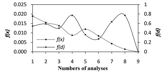
Figure 3.  variations in terms of the analysis numbers.

Figure 4. Network 2 [15].

Figure 5. Change of the pressure and demand fitness in various analyses.
than the base demands, are removed from the list of unknown demand nodes. In the second stage, calibration is performed for the 19 remaining nodes, which leads to elimination of 13 nodes after five repetition of the analysis. The third stage begins with only six nodes. After three more analyses, three other nodes are eliminated. The final calibration leads to leak detection in node number 16 where the real leaky node is located. In comparison with given results in [32], this method found the exact location and amount of leakage through SSEM with fewer observations. Figure 5 indicates no correlation between demand and pressure fitnesses.
The demand fitness remains constant during all the 12 analyses, however after removal of 11 nodes, the calibration is improved rapidly. This is visible in different stages. In order to investigate the variation of Hsim and Hobs, the simulated and observed pressures in four nodes are presented as shown in Figures 6(a) and (b). Figure 6(a) shows the simulated pressures of the first stage. In this figure, the line of perfect agreement between the observational and simulated results is depicted. It is clear that in the first analysis, there are some differences between simulated and observed pressures, while in Figure 6(b) at the final analysis, a complete agreement between them can be observed. Figure 7 shows changing the demand in the node number 16 in various analyses. Demand at node 16 is equal to the base demand at the beginning i.e. 50 l/s, however in the third stage it taken a quantity of 75 l/s which is equal to the actual demand.

Figure 6. Variation of simulated pressures for (a) first analysis and (b) the 20th analysis.

Figure 7. Changes of nodal demands in node number 16 in 16th analysis.
Although in the 15th analysis, the nodal demand is 75 l/s, it should be noted that the demands of other nodes does not matched with true values.
Reducing the searching domain is one of the most significant parts in SSEM. In this network, the numbers of unknown demands are 30 which are equal to the numbers of nodes. For each nodal demand the searching domain is within the interval of 25 - 75 l/s with an increment 5 l/s. In other words, there are 11 options in each node to be selected as its demand. Then the searching ranges in the beginning, first, second and third analysis will be equal to 1130, 1119, 116 and 113 respectively. This shows that step-by-step elimination of the variation parameter options lead to fast convergence of the solution. In the other words, at the final stage, the optimum result will be found among 1331 different states. It means, limiting the search range has eliminated many options which have approximate fitness as well as deceptive results.
3.3. Case 3: Experimental Model
To evaluate the explained methodology, an experimental model is constructed at the hydraulic laboratory of Ferdowsi University of Mashhad, Iran. The height and width of this network are 3.70 m and 10.30 m, respectively. It is equipped with thirty-one pressure measurement positions and eight demand taps for leakage simulation in six loops. Demand can be taken from nodes 1 to 8. In addition, it is equipped with water returning pipes, a pump, a storage tank, and a volumetric measurement tank. Figure 8 represent the different part of laboratorial model consist of: (a) the network; (b) a pressure transducer; (c) pump and flowmeter; (d) volumetric measured tank and finally; (e) a sample of recorded pressure data.
Also, Figure 9 shows the network modeled in EPANET software. Pressure transducers have a total pressure range from 0 to 5 bar and accuracy of 1% of full range. The data collecting system is composed of an eight channel acquisition board, six pressure transducers, and a PC. Pipes are made of PPRC (polypropylene random copolymer). The pipes inner diameters in the loops and branches are 16 and 10 mm, respectively. Each pipe is equipped with a globe valve regulate the flow in the network. A scaled tank measures the nodal consumptions, while an electronic flowmeter records the total inflow of the network with accuracy of 0.03 l/s.
The genetic optimization parameters consisting of the population, fitness tolerance (maximum acceptable fitness) and maximum number of iterations are 50, 0.00001 and 50,000, respectively. Also the node demand is ranged between 0 - 1 and increment by 0.1. Based on these assumptions, the network is calibrated to adjust 8 unknown demand parameters using 4 observations. Three cases of leakage simulations at nodes number 3, 8 and both of them are investigated (the A, B and C refer to the

Figure 8. (a) Laboratory network; (b) pressure transducer; (c) pump and electromagnetic flwmeter; (d) volumetric mesured tank; and (e) a sample of recorded results.
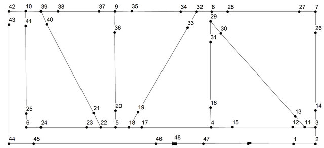
Figure 9. Network model in EPANET 2.
Tables 4-6) and the pressures are measured in nodes 19, 25, 29 and 36 for all the cases; that for each cases, three values of leakages are simulated. The calibration results are presented in the Tables 4-6. In the case A, a leakage in the node 3 with three different deals of 0.63, 0.54 and 0.29 l/s are adjusted. Based on the results which have been shown in the Table 4, in the first stage in order to detect the leakage of 0.63 l/s in the node number 3; the analysis was repeated for three stages and in each stage, some of the non-leaky nodes were found. In the first stage, nodes 6 and 8 were eliminated from calibration process. After three analyses, Nodes 2, 4 and 7 are also omitted in the second stage. In the first analysis of the third stage, a leakage with the quantity of 0.63 l/s at node 3 is shown. Further investigation for Case A are carried out with the leakage quantities of 0.54 and 0.29 l/s. Also in Case B, SSEM has shown its ability to detect the location and quantities of leaky node. As seen in Table 5, the leaky node is Node 8 with the amounts of 0.54, 0.41 and
Table 4. Leak detection results, leak at Node 3.

Table 5. Leak detection results, leak at Node 8.

Table 6. Leak detection results, leak at Nodes 3 and 8.

0.31 l/s. In Case C, Nodes 3 and 8 are leaky. They are detected in the three leakage conditions (Table 6).
The first one; there are an equal leakage of 0.54 in both nodes. In the first stage of calibration after completion of the analyses in three times, Nodes 5 and 7 are eliminated from the list of suspicious nodes. During the second stage, three analyses are performed to omit Nodes 1, 2 and 6. Finally, only one analysis is done to reach the exact solution. The second condition has consisted of the leakage with the quantities of 0.37 and 0.54 l/s at Nodes 3 and 8. Three calibration stages lead to removal of five nodes. At the forth stage, the correct answers through one calibration has been achieved. In addition, the same process is done for the third condition to detect the leakages with an amount of 0.49 l/s and 0.23 l/s at the Node 3 and 8, respectively. The final solution is obtained after four stages.
4. Conclusion
In this paper, the leakage detection in a WDS is investigated using calibration of the nodal pressure in the steady state condition implementing GA optimization. The results have shown that leakage detection in a network, using pressure calibration in the steady state condition, is possible, however it needs a large number of the nodal pressures as observations. Also, the results have indicated that there is no confidence to get the correct solution by satisfaction of the fitness. Moreover, results have shown that changing the crossover and mutation parameters can lead to various answers for the calibration problem, so finding the best results from different options will be a difficult task. However, these several results can be implemented in a novel method presented in this paper entitled “step-by-step elimination method” (SSEM) which has the capability of detecting the leakage in term of its location and quantity. As a novelty of the current paper, to limit the searching domain of possible answer(s), a combination of GA and SSEM is used. By eliminating the nodes which have shown no signal of leakage, the list of leaky nodes is reduced which in turn confines drastically the seeking boundary. By a few number of iteration the locus and magnitudes of leakages can be found. Analyses of two hypothetical networks have shown that identification and elimination of nodes with no signal leakage, easily guide us to the exact location of leaky node with just a few numbers of observation. This cannot be met by GA alone. Also, application of the introduced methodology to a moderate size experimental network model in laboratory has shown its ability to accurately detect the leaky nodes.
REFERENCES
- T. Tucciarelli, A. Criminisi and D. Termini, “Leak Analysis in Pipeline System by Means of Optimal Value Regulation,” Journal of Hydraulic Engineering, Vol. 125, No. 3, 1999, pp. 277-285.
- European Environmental Agency, “First Report on Sustainable Use of Water,” European Environmental Agency, Copenhagen, 1999.
- D. Covas and H. Ramos, “Case Studies of Leak Detection and Location in Water Pipe Systems by Inverse Transient Analysis,” Journal of Water Resources Planning and Management, Vol. 136, No. 2, 2010, pp. 248-257. doi:10.1061/(ASCE)0733-9496(2010)136:2(248)
- A. L. Ekuakille, G. Vendramin and A. Trotta, “Spectral Analysis of Leak Detection in a Zigzag Pipeline: A Filter Diagonalization Method-Based Aalgorithm Application,” Measurement, Vol. 42, No. 3, 2009, pp. 358-367. doi:10.1016/j.measurement.2008.07.007
- T. M. Walski, D. V. Chase, D. A. Savic, W. Grayman and S. Beckwith, “Advanced Water Distribution Modeling and Management,” Haested Press, Waterbury, 2002.
- O. Hunaidi, W. Chu, A. Wang and W. Guan, “Leakage Detection Methods for Plastic Water Distribution Pipes,” AWWA Research Foundation Technology Transfer Conference, Denver, 1999.
- O. Hunaidi, W. Chu, A. Wang and W. Guan, “Effectiveness of Leak Detection Methods for Plastic Water Distribution Pipes,” Workshop on Advancing the State of our Distribution Systems, Denver, 1998.
- Z. Y. Wu and P. Sage, “Water Loss Letection via Genetic Algorithm Optimization-Based Model Calibration,” ASCE 8th Annual Int. Symp. on Water Distribution Systems Analysis, Cincinnati, 2006.
- Z. Y. Wu, T. Walski, R. Mankowski, G. Herrin, R. Gurrieri and M. Tryby, “Calibrating Water Distribution Model via Genetic Algorithms,” AWWA IM Tech Conference, Kansas City, 2002.
- C. M. Rahal, M. J. H. Sterling and B. Coulbeck, “Parameter Tuning for Simulation Models of Water Distribution Networks,” The Institute of Civil Engineers, 1980.
- T. M. Walski, “Technique for Calibrating Network Models,” Journal of Water Resources Planning and Management, Vol. 109, No. 4, 1983, pp. 360-372.
- T. M. Walski, “Case Study: Pipe Network Model Calibration Issues,” Journal of Water Resources Planning and Management, Vol. 112, No. 2, 1986, pp. 238-249. doi:10.1061/(ASCE)0733-9496(1986)112:2(238)
- P. R. Bhave, “Calibrating Water Distribution Network Models,” Journal of Environmental Engineering, Vol. 114, No. 1, 1988, pp. 120-136. doi:10.1061/(ASCE)0733-9372(1988)114:1(120)
- L. E. Ormsbee and D. J. Wood, “Explicit Pipe Network Calibration,” Journal of Water Resources Planning and Management, Vol. 112, No. 2, 1986, pp. 166-182. doi:10.1061/(ASCE)0733-9496(1986)112:2(166)
- P. F. Boulos and D. J. Wood, “Explicit Calculation of Pipe Network Parameters,” Journal of Hydraulic Engineering, Vol. 116, No. 11, 1990, pp. 1329-1344. doi:10.1061/(ASCE)0733-9429(1990)116:11(1329)
- P. F. Boulos and D. J. Wood, “An Explicit Algorithm for Calculating Operating Parameters for Water Networks,” Civil Engineering Systems, Vol. 8, No. 2, 1991, pp. 115- 122. doi:10.1080/02630259108970614
- G. B. Ferreri, E. Napoli and A. Tumbiolo, “Calibration of Roughness in Water Distribution Networks,” 2nd International Conference on Water Pipeline Systems, Suffolk, 1994.
- L. E. Ormsbee, “Implicit Network Calibration,” Journal of Water Resources Planning and Management, Vol. 115, No. 2, 1989, pp. 243-257. doi:10.1061/(ASCE)0733-9496(1989)115:2(243)
- K. E. Lansey and C. Basnet, “Parameter Estimation for Water Distribution Networks,” Journal of Water Resources Planning and Management, Vol. 117, No. 1, 1991, pp. 126-144. doi:10.1061/(ASCE)0733-9496(1991)117:1(126)
- D. A. Savic and G. A. Walters, “Genetic Algorithm Techniques for Calibrating Network Models,” Centre for Systems and Control Engineering University of Exeter, Exeter, 1995.
- T. M. Walski, N. DeFrank, T. Voglino, R. Wood and B. E. Whitman, “Determining the Accuracy of Automated Calibration of Pipe Network Models,” 8th Annual Water Distribution Systems Analysis Symposium, Cincinnati, 2006.
- S. Lingireddy and L. E. Ormsbee, “Hydraulic Network Calibration Using Genetic Optimization,” Civil Engineering and Environmental Systems, Vol. 19, No. 1, 2000, pp. 13-39. doi:10.1080/10286600212161
- D. Kang and K. Lansey, “Demand and Roughness Estimation in Water Distribution Systems,” Journal of Water Resources Planning and Management, Vol. 137, No. 1, 2011, pp. 20-30. doi:10.1061/(ASCE)WR.1943-5452.0000086
- W. Cheng and Z. He, “Calibration of Nodal Demand in Water Distribution Systems,” Journal of Water Resources Planning and Management, Vol. 137, No. 1, 2011, pp. 31-40. doi:10.1061/(ASCE)WR.1943-5452.0000093
- T. Koppel and A. Vassiljev, “Calibration of a Model of an Operational Water Distribution System Containing Pipes of Different Age,” Advances in Engineering Software, Vol. 40, No. 8, 2009, pp. 659-664. doi:10.1016/j.advengsoft.2008.11.015
- T. M. Walski, S. G. Lowry and H. Rhee, “Pitfalls in Calibrating an EPS Model,” The Environmental and Water Resource Institute Conference, Minneapolis, 2000.
- J. Almandoz, E. Cabrera, F. Arregui, E. J. Cabrera and R. Cobacho, “Leakage Assessment through Water Distribution Network Simulation,” Journal of Water Resources Planning and Management, Vol. 131, No. 6, 2005. pp. 458-466. doi:10.1061/(ASCE)0733-9496(2005)131:6(458)
- T. M. Walski, W. Bezts, E. T. Posluszny, M. Weir and B. E. Whitman, “Modeling Leakage Reduction through Pressure Control,” Journal of the American Water Works Association, Vol. 98, No. 4, 2006, pp. 147-155.
- B. Fazel and M. F. Maghrebi, “Detecting Leaks in Urban Water Supply Networks with Field Measurements of Pressure Node (Case Study Golbahar City),” 8th Iranian Hydraulic Conference, 2009.
- J. H. Holland, “Adaptation in Natural and Artificial Systems,” The University of Michigan Press, Ann Arbor, 1975.
- J. P. Vitovsky, R. S. Angus and F. L. Martin, “Leak Detection and Calibration Using Transients and Genetic Algorithms,” Journal of Water Resources Planning and Management, Vol. 126, No. 4, 2000, pp. 262-265. doi:10.1061/(ASCE)0733-9496(2000)126:4(262)
- Z. Poulakis, D. Valougeorgis and C. Papadimitriou, “Leakage Detection in Water Pipe Networks Using a Bayesian Probabilistic Framework,” Probabilistic Engineering Mechanics, Vol. 18, No. 4, 2003, pp. 315-327. doi:10.1016/S0266-8920(03)00045-6