Journal of Water Resource and Protection
Vol.4 No.11(2012), Article ID:24486,14 pages DOI:10.4236/jwarp.2012.411111
Seawater Intrusion and Salinization Processes Assesment in a Multistrata Coastal Aquifer in Italy
Department of Civil, Building and Environmental Engineering (DICEA), Sapienza University of Rome, Rome, Italy
Email: giuseppe.sappa@uniroma1.it
Received August 18, 2012; revised September 19, 2012; accepted October 10, 2012
Keywords: Coastal Aquifers; Geophysical Methods; Environmental Tracers; Salinization; Salt-Water/Fresh-Water Relation; Italy
ABSTRACT
This paper presents the results of the investigations, driven by different techniques, including environmental tracers and geophysical methods, in the aim of better understand the causes of the current salt-water intrusion in the Pontina Plain, in the south of the Lazio Region (Italy). In the last 50 years many investigation campaigns have been carried out to evaluate the evolution of salt-water intrusion. This is an area with a strong man-made residential and tourist impact and, in the some cases, it is characterized by intensive agricultural practices. Therefore, it can be affected not only by salt-water intrusion, but by the salinization of its groundwater also due to other factors. All these factors have led the Pontina Plain to a groundwater situation which makes the groundwater resource management and the planning of their future exploitation very difficult.
1. Introduction
The test site is the southern coastal plain of the Lazio Region (central Italy). It is an area of about 80 km2, most of which has been characterized by coastland and wetland since the beginning of the previous century. In the last fifty years, when the wetland was turned into a plain, many man-made activities started operating such as industrial firms and farms producing most of the fruits and vegetables consumed in the central regions of Italy. The total crop water requirement is about 20 × 106 m3/a, mostly from groundwater; and the area is nowadays crossed by two main systems of irrigation channels in order to increase such yields.
In this damp area, however, seasonal droughts of different intensity are mainly responsible for the variability in the crop yield. The not controlled overexploitation of groundwater and the release of contaminants is slowly, but continuously, leading to the deterioration of this resource. The main concern in the Pontina plain is the remarkable extension of kiwi and mais growing in the last twenty years, which is having a major impact on this resource. Thanks to the favourable climatic conditions and to the availability of irrigation water, these products generate high profits. However, they significantly increase the total water consumption per year and require nitrate fertilization of the soil.
2. Geological and Hydrogeological Framework
The area is included in an ancient tectonic hollow, over 800 meters deep, and covered by recent Quaternary deposits made of sands, silts and clays. More ancient outcroppings are located along the South-West coast and are represented by organogeous limestones or Pliocene and Pleistocene clay. Stratigraphic data collected from deep boreholes and geophysical investigations show that above the Mesozoic-Cenozoic limestone deposit, characterized by normal fault sets, the following sequence is found [1]:
§ Upper Pliocene clay passing to calcarenite in the sectors closer the Lepini ridge.
§ Lower Pleistocene clay—Middle Pleistocene littoral deposits passing to saltier transitional deposits. These sediments contain large amounts of reworked pyroclastic deposits.
§ Marine and transitional clays, sands and gravels deposited during the Upper Pleistocene. Northward of the Plain, volcanic activity of the Colli Albani complex was initiated.
§ Large amounts of peat deposited in the continental fluvio-lacustrine basins during the Holocene.
The Pontina Plain sedimentary layers first developed from a marine depositional system into a transitional fluvial-coastal system, and then into a fluvial-continental depositional system (all during the Pliocene-Pleistocene). Therefore, the entire system is characterized by both vertical and lateral variability that is strongly reflected in its hydrodynamic trend.
Hence, from the hydrogeological point of view, the system of the plain is influenced by:
§ The Lepini mountains along the North-Eastern side (lowered by a net of faults);
§ The Ausoni mountains along the South-Eastern side (separated by the Amaseno discontinuity);
§ The Circeo carbonatic block;
§ The Acque Alte irrigation channel along the NorthWestern side that represents a dranaige axis of the two shallow groundwater systems, as it is better described in the following section.
Four different aquifers have been identified. As a matter of fact, there are two shallow aquifers: the first made by sands and the second made by alluvial deposits which are separated from the deeper carbonatic deposit by a clay layer. The Sisto stream represents a drainage axis for these two Quaternary aquifers. In fact, the first, which is a dune aquifer (in the Western zone of Sisto), flows into the sea and it is drained by the lakes, by the sea and partially by the Sisto stream which bounds the Pontina depression in the South-West. The second one, corresponding to the inner band of the coast (to the East of the Sisto), is constituted by fluvial marsh outcropsand it is characterized by a lower permeability (10–6 m/s). The composition of these strata is really variable because of their different hydraulic conductivity. Nevertheless, the groundwater circulation can be considered unique, thanks to the water exchange through the different strata. The thickness of these layers cannot be defined because of the geological complexity of this structure which makes it very variable from one point to the other. The fourth and minor aquifer is a suspended one, and it is located be- tween the sea and the litoral sandbank (dunal cordon), characterized by a low storage coefficient.
3. Materials and Methods
The aim of the present work is the recognition of evolution and genesis of groundwater salinization by the application of different investigation techniques. This target have been reached by the comparison of the results coming from the application of the different methods:
v Analysis of the stratigraphic reports on the local scale of the test site, which has been fundamental in order to know each useful variation in the lithotypes and simplify the stratigraphic complexity of the study area.
v Vertical electrical soundings (VES) has been carried out to identify the evolution and the trend of saltwater intrusion, in comparison with two previous geoelectrical fields.
v Temperature and conductibility logs have been interpreted to make temperature and conductivity profiles along vertical and horizontal sections, which have been very useful in detecting the flow systems, the preferential groundwater pathways and the salinization origin.
v Chemical and isotopic analyses were helpful in identifying the presence of different salinization.
v Analysis of crop distribution which highlighted the role and the burden of agriculture (and the effects of the policies linked to it) on the current salinization.
The data for this study were obtained from many public and private archives (regional and provincial administrations, universities, etc.). The most important are the Regional Basin Authority of the Lazio Region, the Latina Province, the APAT (National Agency for the Environmental Protection and for technical services) and the ARPA Latina (Regional Agency of Environment Protection). In detail:
a). 4891 stratigraphic reports.
Most of them have been obtained from the Data Archive of the Regional Basin Authority of Lazio. The information about the deepest wells has been obtained from the APAT (Agency for Environmental Protection and Technical Services) archive under Act 464/ 84.
b). 91 VES utilizing the Schlumberger electrode array.
This field measurements have been carried out by the DICEA (Department of Civil, Construction and Environmental Engineering of “Sapienza”—University of Rome) in the months of November and December 2003 and January 2004. This field survey started from the results of two previous geophysical investigations carried out in 1952 and in 1969 by the Compagnie Général de Géophisique.
c). 45 logs meter by meter (CTD data, TDS and PH measures).
These data were obtained from a DICEA field measurement, during the winter 2003-2004.
d). 58 water test results.
32 of them refer to water samples collected by DICEA in three different measurement fields:
§ March - June 2003 (11 wells);
§ November - December 2004 (20 wells);
§ October 2006 (11 wells);
The additional 26 sources are the results of a monthly monitoring carried out by ARPA (Regional Agency for Environmental Protection) for the years 2003- 2004-2005.
e). 15 isotopic analyses.
11 of them on water samples collected by DICEA in during December 2006:
5 are the results of three previous measurement fields of DICEA (April 2002-March 2003-May 2005).
f). A land use coverage for the years 2001-2002 integrated with LANDSAT ETM + images acquired on June 9 2001, December 2 2001, February 4 2002 and August 15 2002.
4. Data Processing
4.1. Stratigraphic Data Processing
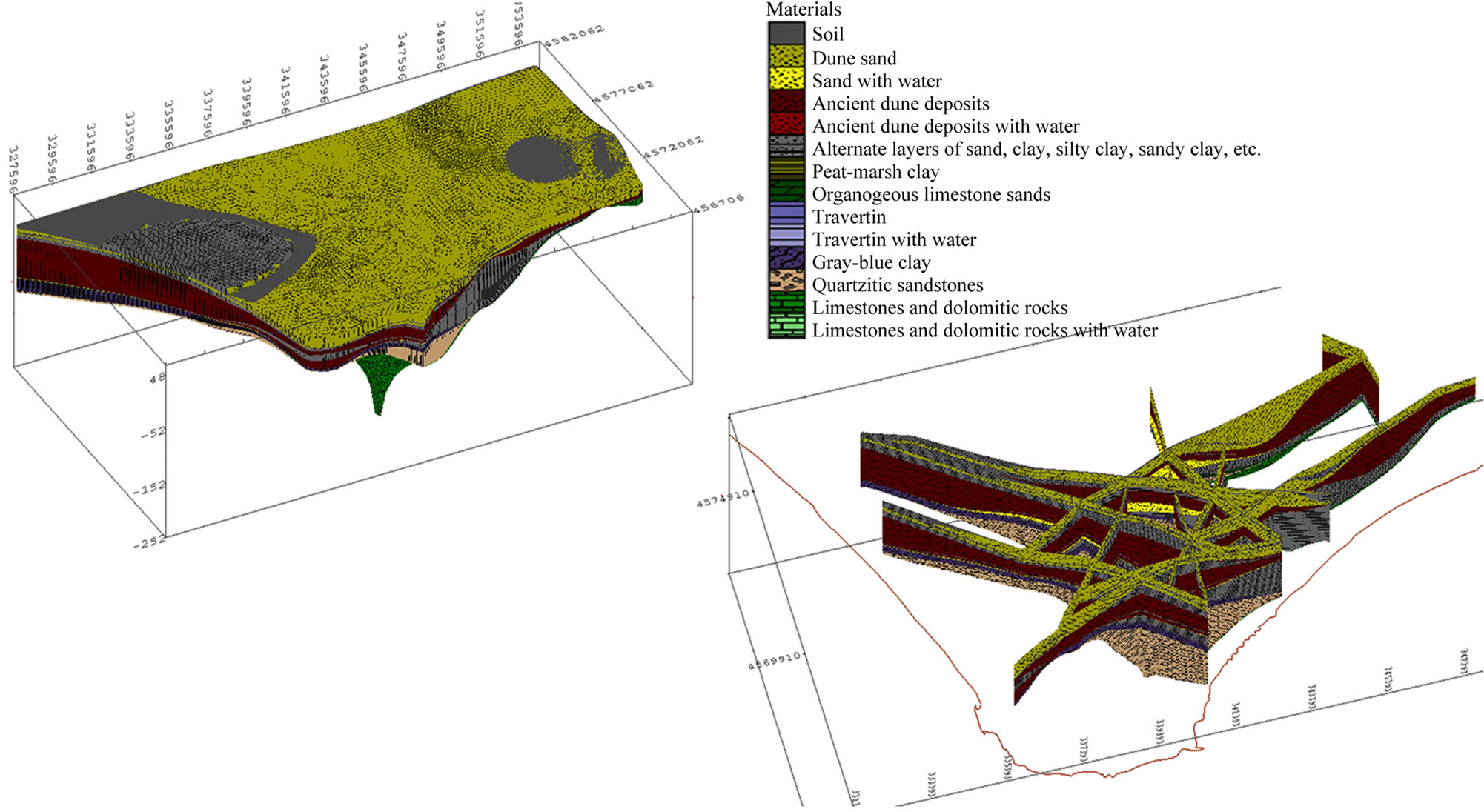
In order to provide an in-depth analysis of the available data on the different layers, a 3D model of the test site stratigraphy was built. The first step was to collect data from public or from private database (regional and provincial administrations, universities, etc.) and to build a MS access database to catalogue and digitize all information about each available drilling. The second step was to check the data reliability (according to their geographic position, accuracy and consistency across the archives) and to match them in a single format. The different drillings were harmonized by joining lithotypes with similar hydrogeological characteristics in order to create the following macro groups:
§ Soil
§ Dune sand
§ Ancient dune deposits
§ Sand with water
§ Peat-marsh clay
§ Organogeous limestone sands
§ Gray-blue clay
§ Travertin
§ Travertin with water
§ Alternate layers of sand,clay, silty clay, etc.
§ Non-lithified volcanic material
§ Quartzitic sandstones
§ Limestones and dolomitic rocks
§ Limestones and dolomitic rocks with water This approach and the use of GIS feature objects (points as drillings, and a polygon as the area boundary) made it possible to build a conceptual model of the aquifer system in the GMS Map Module, defining the boundary conditions, the sources/sinks, and the material property zones. The information was stored on a project-byproject basis. For each project, the number of boreholes or wells was entered, and for each boring samples has been specified at any number of depths. The scatter points were then used to interpolate a surface for each horizon. At each step, a solid was created for the current horizon and all the previously defined solids were subtracted from that solid, thus resulting in an incremental build up of the stratigraphy from the bottom to the top. The resulting solid is shown in Figure 1.
4.2. Vertical Electrical Soundings: Results
The vertical electrical soundings were carried out to identify the depth, thickness, and continuity of the aquifers in the winter of 2003-2004. The analysis started from the results of two previous geophysical investigations conducted in 1952 and in the late 60’s, when 91 VES were carried out in the same location and with the
 (a) (b)
Figure 1. 3D model of test side stratigraphy (a) and cross sections (b).
same aim. This analysis was carried out in November and December 2003 and in January 2004. It consisted of 82 VES utilizing the Schlumberger electrode array. The maximum current electrode (AB) separation was 800 - 1000 m, depending on the accessibility of the soil for expanding the electrodes, also in order to avoid crossing the power lines or the sewerage/water net pipelines when expanding the profile lines and to obtain a better description of the features of the aquifers. In fact, the investigation depth ranged from 120 to 200 m below the ground surface.
The field geo-electric data—in the form of AB/2 (semidistance between the current electrodes)—and the apparent electric resistivity values were plotted on log— log paper in the field, to confirm their reliability in view of their processing and interpretation. The analysis of these curves gives a rough representation of some important experimental results. Moreover, the data from all soundings were interpreted and then utilized for building mean resistivity contour maps at AB = 60 m, at AB = 1000 m (each of them for both periods: 1967 and 2003) and percentage difference maps. They were calculated on the basis of the different field surveys according the following formula (Equation (1)):

They bring out the horizontal extent of the saline water intrusion and the arrangement of fresh water aquifer zones. The legend used for both of them shows the % resistivity increase (e.g. 20%, 30% etc.) or decrease (e.g. –70%, –80%), pointing out to a rise in salt contamination. An apparent resistivity map built considering AB = 60 m (1967) has shown that in the area located between Circeo and Terracina, the resistivity values decrease Eastward passing by a range of 50 - 70 ohm·m. North of S. Felice Circeo, to 5 ohm·m between Borgo Ermada (close to Terracina) and the sea; while, in the area North of Circeo, the resistivity values decrease from the coast inwards. Recently this value has reached more than 50 ohm·m. The same map—built on the 2003 data—has shown a larger conductivity area North of Terracina: resistivity below 40 ohm·m is found in the whole Eastern area of S. Felice Circeo. As mentioned above, Figure 2 was built by comparing the two maps:
This map reports the percentage difference of the re-
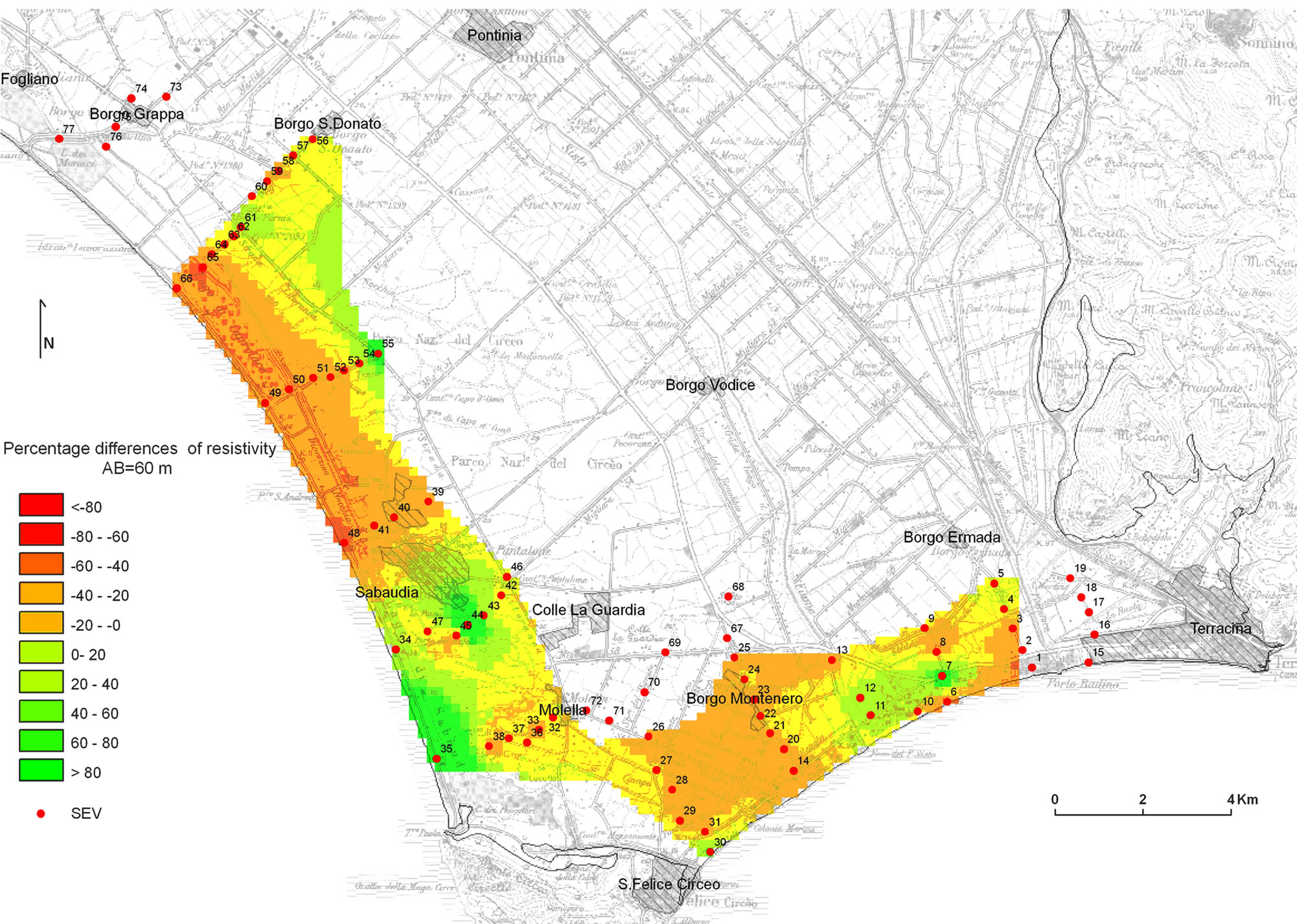
Figure 2. Percentage differences resistivity map by AB = 60 m (1967-2003).
sistivity distribution in the last thirty years for a shallow range of depth between 10 and 30 m and shows a widespread resistivity decrease, with peaks high to 80% in some VES. The lowest values were obtained along the Sabaudia shoreline and on the Western area of Terracina. A particular emphasis should be laid on the situation identified by the sounding data at VES 48, which highlights a decrease by 750 to 35 ohm·m and indicates the elevation of the transition zone. The apparent resistivity map with AB = 1000 m (1967) is related to a survey depth of about 200 m. The lowest resistivity values are located along the Northern coast of Circeo, while the highest at VES 34 and 30. This map, obtained with up-to-date sounding data (2003), shows a similar situation, with very low values in the North and along the coast between S. Felice Circeo and Terracina.
The % differences clearly reveal a decrease in the resistivity value by 20% - 60% along the band between Sabaudia and area North of Circeo (Figure 3).
The highest resistivity values—with 60% - 80% peaks —were registered at VES 30-31 East of S. Felice (T. rre Olevola) and at VES 6-7-10-12 West of Terracina (Porto Badino). In fact, they are located in areas with a high number of man-made activities such as tourist infrastructures. As described later, there was a remarkable increase in resistivity in North-East of the Circeo mountain. Moreover, this trend is different with respect to the one observed in the same area but with a shallower investigation (with AB 60). While the resistivity maps show the horizontal extent of saltwater intrusion, the cross section gives the vertical extent of this phenomenon. Six geological interpretations were obtained from geophysical parameters across the shore line between Terracina and S. Felice Circeo; another six were made North of Circeo. As to the first group of sections, the older field survey of the 60’s showed only one resistant complex and salt water intrusion only in the area closer to the coast; instead, the recent field survey identified a more superficial conductor layer and a sublayer characterized by a resistivity of 2 - 5 ohm·m, i.e. a saline/ brackish one. On the whole, it revealed an elevation of the conductor sublayer vs the situation of 1967. Looking at the second group of sections, it was possible to observe that the resistivity of the sand formations along the coast was lower (1 - 2 Ohm·m) than the 1967 value (3 - 5 Ohm·m) because of the saturation of sand with saltwater.
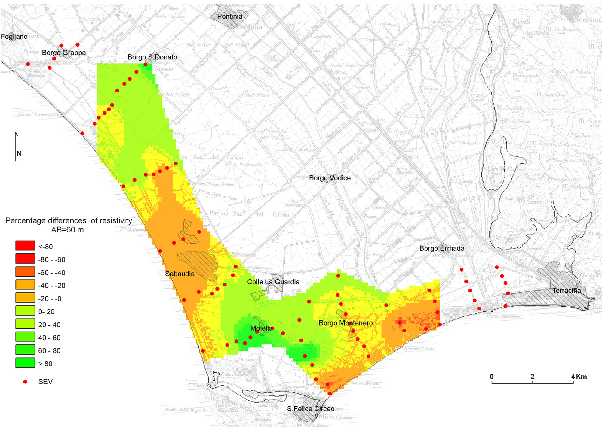
Figure 3. Percentage differences resistivity map by AB = 1000 m (1967-2003).
4.3. Temperature and Conductivity Sections
Groundwater samples (CTD data, TDS and PH measures) were collected from 45 wells, at a depth ranging between 40 - 100 m. For each sample, a meter by meter temperature and a conductivity log profile, and TDS patterns were measured, using the ProfiLine LF 197 sound. By interpolating these data on horizontal and on the vertical plans, temperature and conductivity contour maps were designed to analyze the actual seawater intrusion or salinization processes at different depths. The whole study area revealed conductivity values ranging between 300 and 3600 μS/cm, and a temperature between 14˚C and 18˚C. In particular, by studying the temperature profiles, four different situations were identified:
ü A constant temperature (no gradient) on the whole hydric column probably related to a prevalent vertical circulation component;
ü A positive temperature gradient, i.e.;
ü Temperature rises with the depth; in this case the component of the flux is prevalently horizontal and it is indicative of the extent of the water mobility. The horizontal flux determines the minimum variation in the conductive thermal field and it tends to reach a thermal equilibrium with the surrounding environment;
ü The negative temperature gradient, which means that the temperature decreases in a irregular way with depth, indicating the presence of a gradually faster circulation according to the depth increase. The irregularity may be due to the presence of preferential levels;
ü The gradient is alternately positive or negative, indicative of a complex situation.
Most of the wells investigated showed a trend characterized by ΔT/Δz < 0 or ΔT/Δz = 0. It was not possible to recognize a single cause of this retrograde trend in the temperature, because of the superimposition of different factors. The registered variation is usually 1˚C/100m, except for some wells with variations of 2 or 3 degrees and even of 4˚C/100m in the case of well n. 34. The wells 13, 17, 19 and 39 belong to the second group, i.e. ΔT/Δz > 0. The first three are located in the South-West area and along the same hypothetical axis. This may be due to a slow circulation or to saltwater intrusion. In this case, the comparison between the temperature and conductivity logs was instrumental in making a distinction between them. The wells characterized by both ΔT/Δz < 0 and ΔT/Δz > 0) are concentrated in the central area, North of Circeo; these variations may depend on the extreme heterogeneity of the local stratigraphy, which is more complex than in the West and East areas.
By interpolating the logs described above on the horizontal and vertical plans, temperature and conductivity contour maps were designed to study the actual seawater intrusion or salinization processes at different depths.
The interpretation of the log data was carried out by reconstructing the trend of the isotherms along meaningful vertical (and horizontal) sections.
The most representative ones both on the West and East are reported.
5. Discussion
5.1. Temperature and Conductivity Cross Sections
In order to correctly read the results of the thermal and conductivity patterns along the sections plotted on the map in Figure 4:
It has been necessary to make a double check:
ü Cutting the stratigraphic slices (by the solid described above) along the same axis.
ü Adding other stratigraphic fences slices by cutting them along the VES cross section.
The most widespread distribution of saltwater intrusion is evident in the area of Terracina, that is Eastern area of the test side.
Here two sections are particularly important 8 (Figure 5(b)). The first was built by interpolating conductivity and temperature data relative to wells n. 46 and n. 47. The second by interpolating data of wells n. 47 and n. 45. The stratigraphic succession is the same for both of them, but the saltwater intrusion is found at different depth levels: between –25 and –50 m, the first, and between –5 and –25 the second. In both cases, the conductivity values reach 3000 μS/cm. The comparision with the geoelectric section C (Figure 5(c)) confirms the existence of a sandy layer between 0 - 40 m saturated with salt water and with a resistivity range between 1 - 15 ohm·m.
5.2. Planar Sections
Two planar sections were built for the central area featuring Montenero (E), Colle La Guardia (N), Molella (W) and Circeo (S), showed in Figure 6.
The interpolated layers were obtained by projecting the temperature values corresponding to –5 m and to –20 m a.s.l., read on the vertical sections obtained from the previous interpretation of data points. It is possible to recognize the inland saltwater intrusion from the coast along two main axes, crossing near wells n. 16 and 38 respectively, with the highest temperature of 17.5˚C between 15 and 20 m from the ground level. The fresh water cone characterized by a very low temperature located in the central area is very important; in fact, it confirms the previous hypothesis, i.e. the presence of a preferential circulation of cold water coming from the Circeo. Moreover, a detailed stratigraphic analysis showed the presence of “rock with water” due to a fresh flow colder that the others in the wells present in the neighboring area.
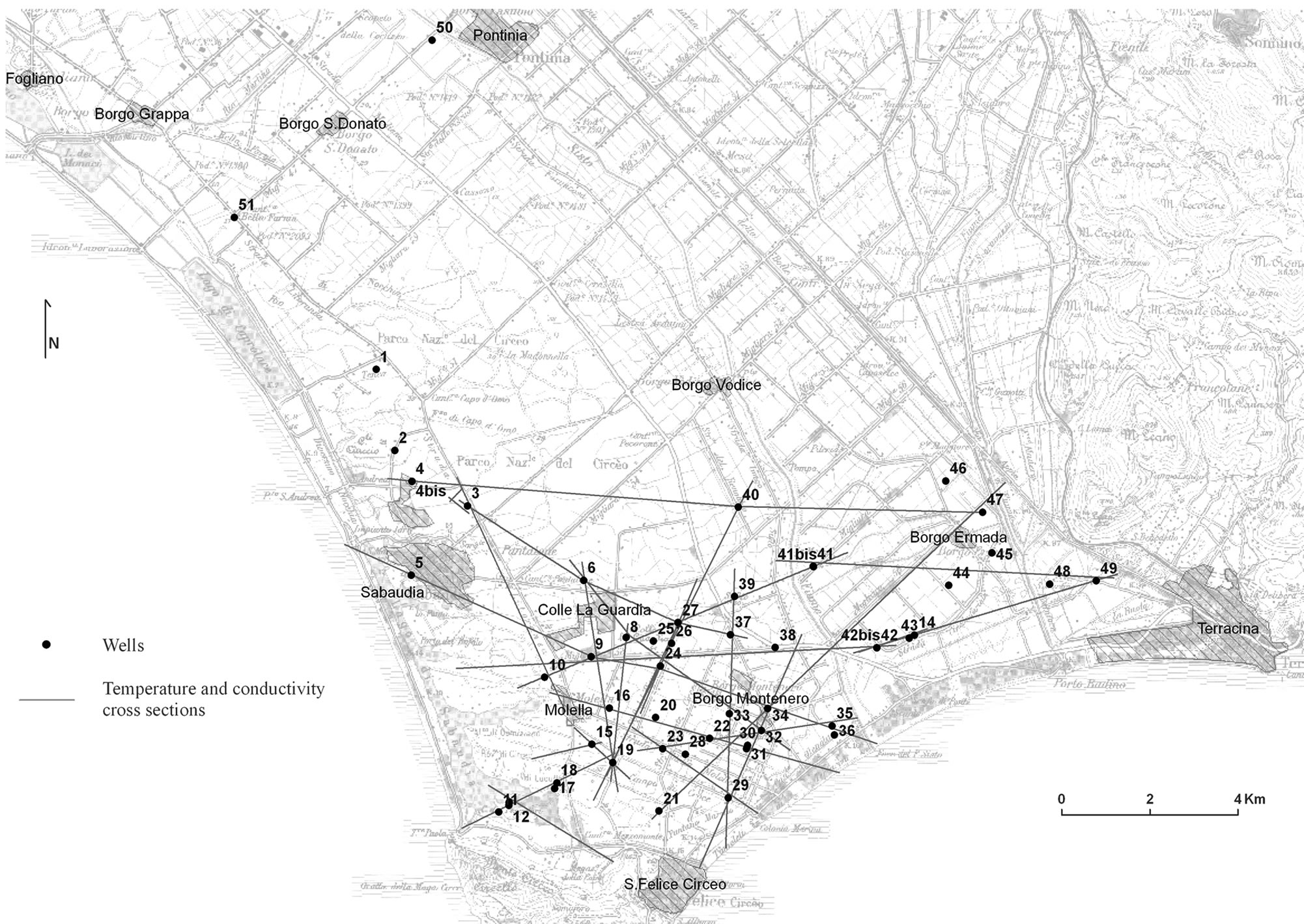
Figure 4. Location of wells and temperature-conductivity cross sections.
5.3. Chemical Water Features
A series of geochemical processes is taking place in the fresh water-seawater contact zone of the Piana Pontina aquifer, which is altering the freshwater and seawater mixture with respect to its theoretical composition. The analysis of the chemical and isotopic composition of groundwater sampled in the coastal plain produced useful information to recognize the origin of salinization or to exclude saltwater intrusion.
These processes are not easily specified since they vary and overlap both in time and space and because they are more active in the zone of mixing or where salinity is higher. Often, the most visible process is cation exchange: it takes place between the clay and the groundwater and is quite clear in the detritic sediments as reverse exchange (removal of Na+ from solution) between Na+ and Ca2+-Mg2+ ions. In a coastal aquifer direct exchange is indicative of flushing, while reverse exchange is evidence of active marine intrusion. Other processes include dolomitization—dedolomitization driven by sulfate solution (causing excess of calcium, magnesium and sulfate), sulfate reduction (deficit of sulfate), precipitation of gypsum coupled with ion exchange during the early stages of seawater intrusion/salinization. The ion-exchange efficacy and the superimposition of other salinization processes were suggested on the basis of the following considerations. Cross plots of major concentrations vs. chloride concentration for all available samples showed that ion concentration is not in line with the theoretical conservative mixing lines, which can be calculated between a water sample and the present seawater. The first is the freshest among the fresh available samples analysed and taken as fresh water end member (FW); the second is a sample collected from the shore close to Terracina and considered as salt end-member (SW). The calcium content is very high along the SW-FW mixing line in the majority of the samples analyzed. This is due to some processes determining the enrichment of calcium in solution, both when salinization is present or not. By observing the Mg vs Cl content, there is evidence of excess magnesium in comparison with the SW-FW conservative mixing lines. This excess turns into a deficit only at higher mineralizations Na vs Cl and K vs Cl follow the same trend, showing excess contents for the highest mineralizations and deficits for the lowest ones. The excess of Ca reveals the overlapping of many proc-
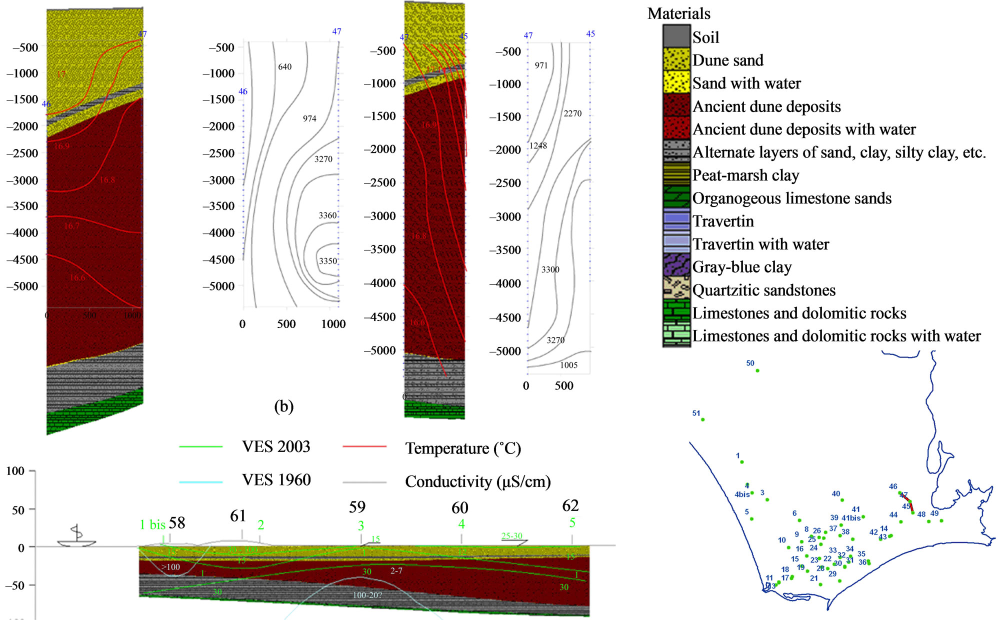 (c) (a)
Figure 5. Location of wells (a), temperature and conductivity cross sections (b), geoelectrical cross sections (c).
esses. In fact, the Ca vs SO4 graph shows that Ca increases in line with sulfate increase, but not in line with the conservative mixing line or with the stoichiometric ratio Ca:SO4 (1:1). This is the effect of a combination of different processes such as CaSO4 dissolution, ion exchange, carbonate dissolution (calcite, dolomite, magnesic calcite etc.). In the graph below, bicarbonate increases in line with the mineralization level but decreases in the presence of a sulfate solution and ion exchange and when Ca begins to rise. The samples PP collected during 2003 generally follow the mineralization levels: if Ca increases, HCO3 increases. By looking at the whole data sample in a graph (Figure 7).
it is evident that the sulfate enrichment process is also present in the Lepini and in the Ausoni water samples. This enrichment can be explained only by the CaSO4 solution (as in ID1, ID10, ID12, PP12, ID27) or by CaSO4 followed by NaCl (like in evaporitic salt). In fact, the SO4/Cl ratio does not correspond to the SW-FW mixing line one (Figure 7(b)). There are no pyrites in the soils of this area. Therefore, the presence of other processes which adds sulfate for the oxidation of sulfates is to be ruled out. The Ca vs SO4 (Figure 7(c)) graph with the whole data set (PP samples with PP04 as fresh water end member, ID samples with ID 19 as salt end member and springs samples) better explains these concepts: if the Ca concentration changes in a high value range of 0.5 - 3 meq/L, the cause is an incongruent dolomite dissolution and/or an ionic exchange with sodium. The Na-Cl diagram (Figure 7(a)) shows that only PP (10, 13, 11) clearly has an Na deficit, while other samples such as the Ausoni springs have a very high content of Na, thus indicating that, in some cases, sulfates and clorures come from the formations ant not from the sea. In order to determine the behaviour of these cations and to identify the processes that modify the theoretical content, the calculation of the ionic delta is presented for each of the cations analysed. The calculation of the ionic deltas (Δ) is based on the comparison between the actual concentration of each constituent and its theoretical concentration for a freshwater-seawater mix derived from the Cl concentration of the sample [2]. Equation (2) is:

where ΔCi is the ionic delta of the ion i, Ci,sample is the measured concentration of the ion i in the sample, and Ci,mix is the theoretical concentration of the ion i for the conservative mix of freshwater and seawater. The theoretical mix concentration was calculated by considering the seawater contribution from the Cl concentration in the sample (CCl,sample), from the freshwater Cl concentration (CCl,f) and from the seawater Cl concentration
 (a)
(a) (b)
(b)
Figure 6. Temperature planar sections: –5 m a.s.l. (a), –20 m a.s.l. (b).
 (a) (b) (c)
Figure 7. Na vs Cl plot (a), SO4 vs Cl plot (b), Ca vs SO4 plot.
(CCl,sea). Equation (3) is:

This seawater contribution was used for calculating the theoretical concentration for each ion (Equation (4)):
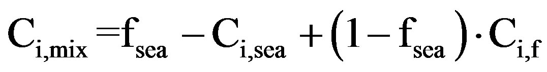
In these calculations Cl can be considered as a conservative tracer: it only comes from the salts in the aquifer matrix itself or from a salinization source and it is not usually removed from the system due to its high solubility [3]. The delta ΔCi will be considered as an excess content if positive or as a deficit content if negative. The map in Figure 8 shows the deviations (excess or deficit) for Na, Ca, SO4, HCO3 and for Ca + Mg vs. Cl, on the left of the Sisto stream:
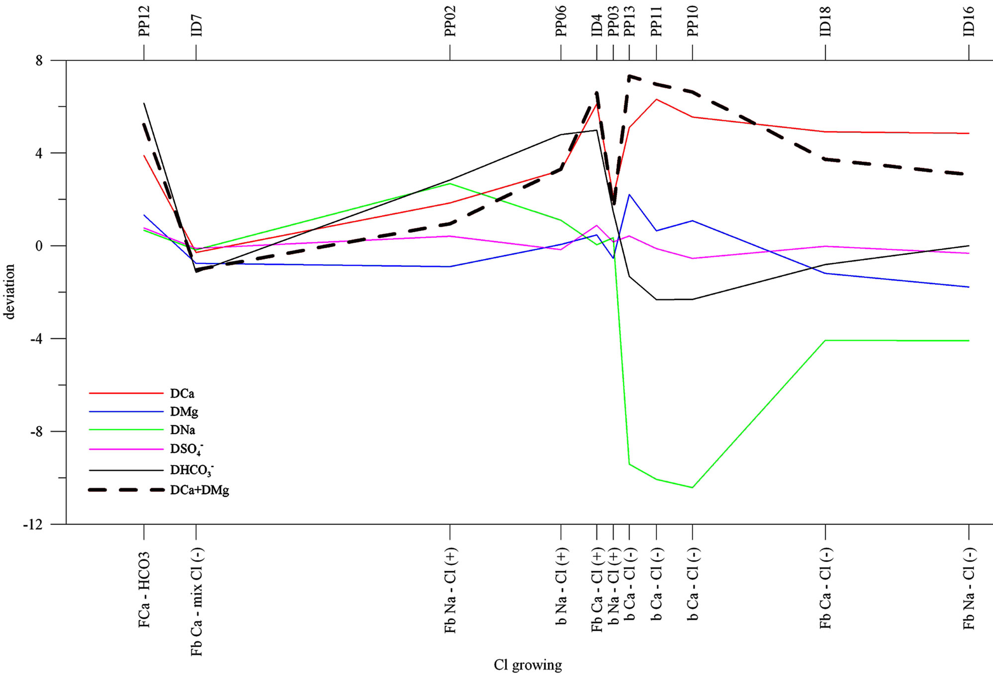
Figure 8. Ionic deviations on the left bank of Sisto stream.
The presence of an ionic exchange is evident for the ID and PP with a higher salt content, especially compareing ΔNa with ΔCa-ΔSO4 which eliminates the effect of the sulfate solution (in fact ΔNa and ΔCa-ΔSO4 are rather specular. The cause is different for PP and for ID. In fact, given the distance from the sea, PP should be salinized due to past salinization, to the washing away of clays or to other processes but it cannot be associated to the present saltwater intrusion from the coast. Instead, the salinization of ID 18 an ID 16 is surely correlated to it, also considering the Ca, Na and K vs. Cl patterns. The samples taken from the right hydrographic bank of Sisto show a ionic change starting from ID 14. The hydrofacies are typical of salinization but for ID 9-10-34 it is necessary to check the temperature and the conductivity profiles. Nevertheless by considering ΔCA + ΔMg – ΔSO4 – ΔHCO3 as the total excess/deficit of calcium and magnesium purified from the effect of the sulfate solution and of the bicarbonate equilibrium, it is possible to obtain an indicative value of Na and consequently of the extent of the cationic change.
5.4. Isotopic Analysis
Eleven water samples were taken in December 2006 and another 5 from three previous measurement fields (April 2002, March 2003 and May 2004), were analyzed for stable isotope (18O and 2H) contents. Figure 9 shows their details.
Notwithstanding the chronological inconsistency of the available data, the results of the previous surveys were a useful starting-point to interpret the 2006 data. Because of the lack of pluviometric data, the analysis compared the isotopic patterns in the samples located in the plain and in the freshest springs located on the neighboring mountains.
Two samples were selected from the Lepini and the Ausoni springs: one at the lowest altitude and the other at the highest. The first—LP03 (Table 1) with δ18O = –5.23, shows the lowest conductivity value and a recharge at 100 m a.s.l; the second—LP16 with δ18O = –7.58 presents a conductivity value of 296 μS/cm and a recharge not above 1400 m a.s.l. For the purpose of this study, a recharge altitude of 1200 m a.s.l. was chosen. The water line built on the basis of these two samples is in line with the Local Meteoric Water Line for Central Italy suggested by Longinellli and Selmo [4]: with a weighted mean 18O value of –0.2‰/100m. Starting from this line, the levels of the sweetest water samples (collected during October 2006) were evaluated. The

Figure 9. Location of water samples for isotopic analysis.
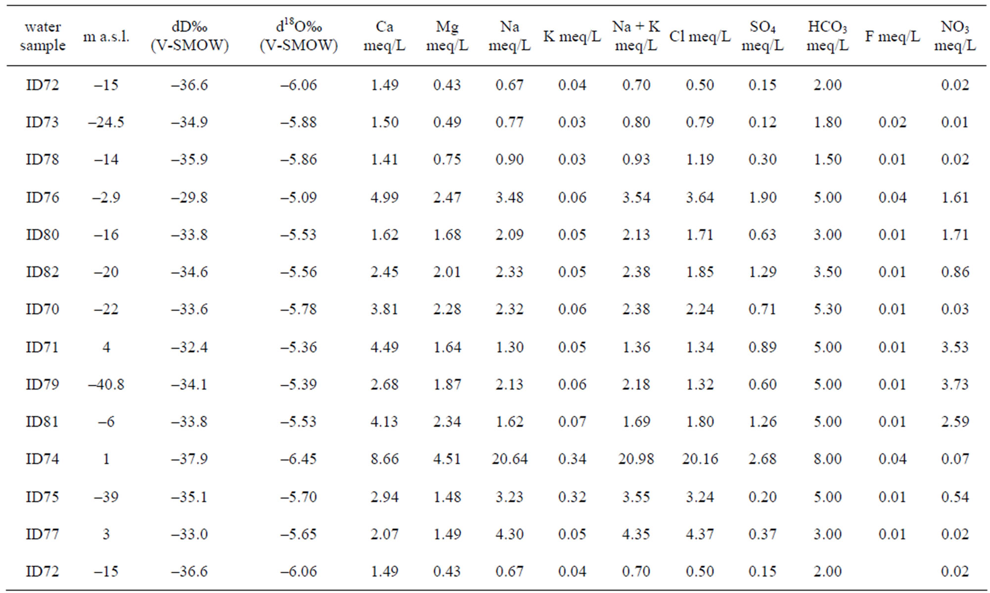
Table 1. Isotopic and chemical features.
Table 1 shows the results.
The most interesting observation of this analysis was that the level of the water samples located in the plain is higher than the one of the dune (where the max level is 36 m a.s.l. at Colle La Guardia). This is true not only on the Lepini and the Ausoni mountains but also in Circeo where it reaches 599 m above the sea. This strengthens the hypothesis of a fresh water feeding coming from Circeo.
In order to analyze the correlations between the isotopic and the chemical features, the whole sample set was clustered on the basis of a defined chemical pattern. Four different groups were obtained according Schoeller diagram: GROUP I-GROUP II-GROUP III-GROUP IV. The data of the stable isotopes referred to the clustering of GROUP I (composed of ID 72 + ID 73 + ID 78 wells) and of GROUP IV one (ID 75 + ID 77 wells) follow the mixing line with a good correlation. By correlating this pattern with the chemical results in the same area, it was possible to confirm that the salinization recorded North of Terracina (where ID 75 and ID 77 are located) is surely due to saltwater intrusion. The same phenomenon was found North of Circeo and also in other areas as shown later.
5.5. Crops Data Manipulation and Graphical Treatment of N and Cl Concentrations
A land use coverage for the year 2001-2002 was used to estimate different levels of nitrogen input. The water test results from the ARPA database for the years 2003-2006 were linked to the information coming from two field measurements of wells (November 2001-December 2003) carried out by this department. The geological data from the Regional archives and from APAT were used to assign the aquifers to the tested wells.
The cropland layer utilized is the one created by Casa R. [5]:, starting from a digital land use map [6]: already available for the study area this was then integrated with LANDSAT ETM + images acquired on June 9 2001, December 2 2001, February 4 2002 and August 15 2002. Moreover, in order to distinguish permanent crops from non permanent ones, a field survey was carried out in April 2005 and some information was extracted from the farmers’ statements submitted to become eligible for the Common Agricultural Policy (CAP) and the Structural Funds subsidies, stored in the database of the state agency AGEA. Moreover, the use of ortophotos helped to check the reliability of the information. Finally a classification map including 17 crop types was obtained. In order to show as crop types and their irrigation requirements are responsible for localized peaks of nitrate concentration, a first step was to build entry matrices for the spatial analysis of data. They were organized in 49 rows (number of available data on wells) and in 6 columns according to the following variables:
1). latitude 2). longitude 3). crop type 4). hectares of each crop type inside a circle with a 400 m radius 5). cropland as a percentage of the total cultivated area inside the circle 6). N concentration 7). Cl concentration 8). Further chemical analysis Later, to draw a map and to show the impact of each crop, it is the different types of data were aggregated in terms of nitrate requirements (kg/ha) and a risk value was assigned according to the classification suggested in the following Table 2. The values of nitrate concentrations, reported in the table, are adopted from [7].
The cropland layer was plotted into 49 circles with a radius of 400 m, with the centre corresponding on each well by using the buffer command. This shows that the impact of nitrogen inputs to the crops which need of it as fertilizer is defined by a circle of 50.24 ha. A centroid with all the information of the polygon to which it belongs was associated to each crop-polygon.
5.6. Spatial Analysis
The methodology for estimating the amount of nitrate stored in the aquifer was based on the results obtained from the spatial analysis undertaken for the purpose of this study. The distribution of nitrate concentrations was analyzed for correlation with the aforementioned vari-

Table 2. Nitrate requirements of crops and dangerous classes.
ables. The Spatial Analysis with the Kernel density function allowed us to build a density map for crops and to study the results obtained by overlapping it with the nitrate concentration map and the map of piezometric decrease (from 1979 to 2003). The Kernel Density calculates the density of point features around each output raster cell. Conceptually, a smoothly curved surface is fitted over each point. The surface value is highest at the location of the point and diminishes with increasing distance from the point, reaching 0 at the [radius Distance] distance from the point. The kernel function was based on the quadratic kernel function described in [8]. The population field was used to weigh some points more heavily than others, depending on their meaning, or to allow one point to represent several observations. To this end, for crop density maps, the hectares with the lowest danger were considered first, and the hectares with the highest danger later, as population field. The following maps indicated a positive relationship between the density of croplands belonging to the dangerous classes n. 4 and 5 and the highest nitrate levels in groundwater (mg/L). In fact, the distribution and density maps of crops and nitrate concentration map show a similar curved surface, in line with the highest and the lowest piezometric surface values in the same locations. In fact, the maps indicated a high density of crops (corn) and high nitrate concentrations in the central area (Borgo Montenero) and along the West coast (Sabaudia). Instead, low concentrations were found in forage fields east of the test site (Borgo Ermada).
6. Conclusions
The integration of results coming from different techniques of field investigation and laboratory analysis, drove to highlight and to map different salinization processes in the Southern coastal area of the Pontina Plain.
The VES investigation showed that seawatwer intrusion grew both vertically and horizontally. In the aquifer, the 2003 VES study showed that seawater came in at two different levels: the first located at about 40 - 80 usl in the more recent sands, while the second at about 100m u.s.l. in the layer of more ancient sands. These two levels have been divided by a thick layer of Plio-pleistocene silts and clayes. The seawater intrusion involved the aquifers and the aquitards, under the fresh water level at a depth of 10 meters for the first aquifer and at 40 meters for the second one. In the horizontal direction, the seawater intrusion was observed for more than 500 m on the West coast and for more than 2 km in the East part. On the other hand, the geoelectrical investigation showed two anomalies that could not be explained without the results of different methods: the resistivity value increased NW of Circeo and it was very low near well no. 39. Temperature and conductivity logs and sections confirmed most of the saltwater intrusion directions suggested by the VES. But they also showed high conductivity levels that could not be due to saltwater intrusion and areas characterized by very fresh and cold waters. The variation of the chemical composition revealed different salinization processes (current and old seawater intrusion, dedolomitization, sulfate reduction and nitrate contamination) and confirmed the hypothesis—strengthened by the isotopic results—that waters coming from Circeo fed the same aquifer affected by saltwater intrusion. This could explain the anomalies identified both by the VES investigation and by the T˚ and C profiles. Moreover, by crossing the stratigraphical results, the chemical characterization and the analysis of cropland made it possible to explain the presence of high conductivity levels not followed by high temperature or low resistivity and, for these reasons, they were not due to salt water intrusion, but to a different source of salinization. The aquifer thickness varies a lot in this area so it was impossible to set up a reliable correlation between the aquifer volume and the distribution of the anion concentrations. Anyway, a comparison of nitrate concentration versus aquifer volume was attempted by extracting some cross sections from the solid described above. Transects like those shown in Figure 9 helped to give an idea of magnitude of the thickness and depth of the layers, characterized by an alternation of sand, clay, silty clay etc. Then, considering the following factors:
§ Depth of the wells—the shallower the well, the higher sensitivity. Deeper wells were protected by the presence of a clay layer, which restricted or hampered the flow of water and of possible contaminants;
§ Soil recharge potential—the sandier the soils, the higher the sensitivity. Sandy soils allow more water to infiltrate from the surface to the subsurface than do silt or clay soils.
It was confirmed that the central and the western areas showed more sensitivity to nitrate contamination because of a high density of crops with high nitrate requirements and of the specific vulnerability of aquifers. In fact, the concentration of nitrate and chloride was correlated with the vertical position of the aquifer within the stratigraphic unit. This suggested that a lower concentration was found when a confining unit was present. Likewise, the profiles extracted from a TIN (Triangulated Irregular Network) interpolated from nitrate concentration values showed a general decline in nitrate concentration with the increase in the soil thickness. This could explain the anomaly also correlated to well no. 39.
REFERENCES
- P. Tuccimei, R. Salvati, G. Capelli, M. C. Delitala and P. Primavera, “Groundwater Fluxes into a Submerged Sinkhole Area, Central Italy, Using Radon and Water Chemistry,” Applied Geochemistry, Vol. 20, No. 10, 2005, pp. 1831-1847. doi:10.1016/j.apgeochem.2005.04.006
- M. D. Fidelibus and L. Tulipano, “Mixing Phenomena Owing to Sea Water Intrusion for the Interpretation of Chemical and Isotopic Data of Discharge Waters in the Apulian Coastal Carbonate Aquifer (Southern Italy),” Proceedings of the 9th Salt Water Intrusion Meeting, Delft, 1986, pp. 591-600.
- C. A. J. Appelo and D. Postma, “Geochemistry, Groundwater and Pollution, xvi + 536 p,” A. A. Balkema, Rotterdam, Brookfield, 1993.
- A. Longinelli and E. Selmo, “Isotopic Composition of Precipitation in Italy: A First Overall Map,” Journal of Hydrology, Vol. 270, No. 1-2, 2003, pp. 75-88. doi:10.1016/S0022-1694(02)00281-0
- R. Casa, M. Rossi, G. Sappa and A. Trotta, “Assessing Crop Water Demand by Remote Sensing and GIS for the Pontina Plain, Central Italy,” Journal of Water Resources Management, Vol. 23, No. 9, 2009, pp. 1685-1712. doi:10.1007/s11269-008-9347-4
- L. Piemontese and C. Perotto, “Carta Dell’uso del Suolo Della Provincia di Latina,” Gangemi Editore, Roma, 2004.
- L. Padovani, M. Trevisan and E. Capri, “Pericolo Potenziale di Contaminazione Delle Acque Sotterranee da Nitrati di Origine Agricola,” Cnrgndci, Regione Liguria, 2000, 55 p.
- B. W. Silverman, “Density Estimation for Statistics and Data Analysis,” CRC Press, Boca Raton, 1986.