Journal of Water Resource and Protection
Vol.3 No.10(2011), Article ID:8135,11 pages DOI:10.4236/jwarp.2011.310085
Nonlinear Deterministic Chaos in Benue River Flow Daily Time Sequence
Department of Agricultural & Bioresources Engineering, Federal University of Technology, Minna, Nigeria
E-mail: martynso_pm@yahoo.co.uk
Received June 21, 2011; revised July 29, 2011; accepted September 3, 2011
Keywords: Deterministic Chaos, Nonlinear Dynamics, Phase Space, Correlation Dimension, Time Delay
ABSTRACT
The Various physical mechanisms governing river flow dynamics act on a wide range of temporal and spatial scales. This spatio-temporal variability has been believed to be influenced by a large number of variables. In the light of this, an attempt was made in this paper to examine whether the daily flow sequence of the Benue River exhibits low-dimensional chaos; that is, if or not its dynamics could be explained by a small number of effective degrees of freedom. To this end, nonlinear analysis of the flow sequence was done by evaluating the correlation dimension based on phase space reconstruction and maximal Lyapunov estimation as well as nonlinear prediction. Results obtained in all instances considered indicate that there is no discernible evidence to suggest that the daily flow sequence of the Benue River exhibit nonlinear deterministic chaotic signatures. Thus, it may be conjectured that the daily flow time series span a wide dynamical range between deterministic chaos and periodic signal contaminated with additive noise; that is, by either measurement or dynamical noise. However, contradictory results abound on the existence of low-dimensional chaos in daily streamflows. Hence, it is paramount to note that if the existence of low-dimension deterministic component is reliably verified, it is necessary to investigate its origin, dependence on the space-time behavior of precipitation and therefore on climate and role of the inflow-runoff mechanism.
1. Introduction
One aspect which hydrologists have been extensively working on is the structure of hydrological processes, such as rainfall and runoff [1]. Even though, during the past decades, a number of mathematical models have been proposed for modelling hydrological processes, there is, however, no unified mathematical approach. In part, this difficulty stems from the fact that hydrological processes exhibit considerable temporal variability; by extension, another part of this difficulty is due to the limitation in the availability of “appropriate” mathematical tools to exploit the structure underlying the hydrological processes [1]. The tremendous spatial and temporal variability of the hydrological processes has been believed, until recently, to be due to the influence of a large number of variables. Consequently, the majority of the previous investigations on modelling hydrological processes have essentially employed the concept of stochastic process. However, recent studies have indicated that even simple deterministic systems, influenced by a few nonlinear interdependent variables, might give rise to very complicated structures (i.e., deterministic chaos) [1]. Therefore, it is now believed that the dynamic structures of the seemingly hydrological processes, such as rainfall and runoff, might be better understood using nonlinear deterministic chaotic models than the stochastic ones. Despite this posturing though, “it is highly improbable that complex natural phenomena may be controlled only by the presence of a chaotic dynamics”; rather, if it is present, it most likely coexists with other types [2]. It is therefore a weaker form of determinism which may be hidden in complex natural systems. As affirmed by Grassberger [3], “the emphasis should not be whether the strongest form of determinism (absence of all random noise) is a good model for the underlying process, but rather whether the weakest form of determinism consistent with other tests can be ruled out”.
Against the backdrop of the dynamics governing river flow, therefore, investigating the existence of a chaotic component and more generally, nonlinear time sequence analysis may be useful in understanding some aspects of the phenomenon of river flow process. This is imperative considering the fact that river flow dynamics is linked both to the climate, through precipitations, radiation, etc., and to the inflow-runoff transformation. Thus, the existence of chaos cannot be excluded a priori. Generally, it should be noted that there are some aspects of the inflow-runoff transformation which may reduce the complexity of the local dynamics of the climate, shading some degrees of freedom and privileging others. For instance, especially, the geometric, hydraulic, and hydrogeological characteristics of the watershed [2], and the topology of the network (e.g., [4-6]), and the presence of aquifers and storage capacities such as lakes should not be ignored a priori. Some of these effects, individually or as a whole, may shade the strong spatial and temporal variability of the precipitations, reducing the number of active degrees of freedom and producing a strong nonlinear deterministic character. This does not mean that river flows are exclusively reducible to a nonlinear interaction of a few degrees of freedom. Even simple hydrological considerations reveal the error of such an assertion [3]. Therefore, what is important is to investigate if the dynamics of the discharges of a river has a dominant chaotic component on which high-dimension linear and nonlinear dynamics are grafted. The theory of nonlinear dynamic systems associated with the concept of strange attractors provides a new technique for time series analysis; this is because in many instances, the time series can be viewed as a dynamic system with a low-dimensional attractor which can be reconstructed using the ‘time delay embedding method’. The dynamic systems theory approach has been applied to analyse weather and climate data ([7-10]). These studies focused on the calculation of the geometric and dynamic invariants of an underlying attractor from a time series of observations, such as the fractal dimension and the Lyapunov exponents. The calculated invariants can be used to diagnose whether the time series is chaotic or not.
In a simple contextual framework, the term “chaos” is used to denote the irregular behaviour of dynamical systems arising from a strictly deterministic time evolution without any source of external stochasticity but with sensitivity to initial conditions. From a physical point of view, the most striking difference between a picture based on a stochastic description and the approach based on deterministic chaos is essentially contained in the very different number of variables, which characterise the system [11]. If, given some irregular dynamics, one is able to show that the system is dominated by a lowdimensional attractor (an attractor is a geometric object that characterises long-term behaviour of a system in the phase-space), then an important physical result is that the system dynamics can be described by only a few modes and hence a small system of ordinary differential equations [11]. This is in sharp contrast to the behaviour of systems dominated by a very large number of excited modes which are in general better described by stochastic or statistical models.
Thus, determining the presence of low-dimensional attractor from time series data has important dynamical implications. Hence, the calculation of the system dimension is one of the steps toward this goal. The central idea behind the application of this approach is that systems whose dynamics are governed by stochastic processes are thought to have an infinite value for the attractor dimension, whereas a finite, low, non-integer value of the dimension is considered to be a strong indication of the presence of deterministic chaos [11]. This assertion is premised on the realisation that stochastic processes are thought to fill very large-dimensional subsets of the system phase-space, while the existence of a low-dimensional (chaotic) attractor implies that only a rather lowdimensional sub-set of the phase-space is asymptotically visited by the system motion. In apt recognition of the issues involved, the central thesis of this paper is to test the hypothesis that the daily streamflow process of the Benue River can be described by a small set of variables; that is, it is low-dimensional. The importance of this can be understood against the premise that such evidence may be useful for developing low-order models that may help to explain whether whatever prevailing variability in the dynamics of the flow process might be linked to low-frequency climatic variability.
2. Materials and Methods
2.1. Hydrology of the Benue River/Data Base Management
In this study, historical time series for gauging stations at the base of the Benue River (i.e., Lower Benue River Basin) at Makurdi (7˚44′N, 8˚32′E) was used. A total of 26 years (1974-2000) water stage and daily discharge data were collected. The Benue River is the major tributary of the Niger River. It is approximately 1400 km long and almost navigable during the rainy season (between July and October). Its headwaters rise in the Adamawa Plateau of the Northern Cameroon, flows into Nigeria south of the Mandara Mountains through the east-central part of Nigeria. There is only one high-water season because of its southerly location; this normally occurs from May to October, while on the other hand, the low-water period is from December to June. Figure 1 explains the
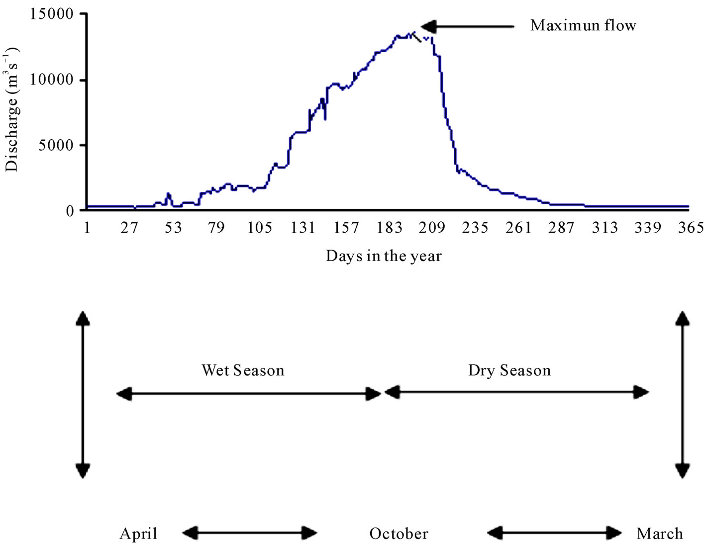
Figure 1. General hydrological year flow regime.
hydrological flow regime of the Benue River in line with the general climatic pattern. There are definite wet and dry seasons which give rise to changes in river flow and salinity regimes. The flood of the Benue River (upper, middle, and downstream) lasts from July to October, and sometimes up to early November.
The mean daily discharges are as shown in Figure 2. Clearly visible are the flood peaks and the seasonal periodicity, with both large and small discharges during the year. Such persistent regimes are related to regional climatic variability. Besides, the autocorrelation and spectral analyses provide the first important indications on the aperiodicity of the signal under examination. Figure 3 shows the autocorrelation for values of the delay time (lag) between 0 days and about 5 years. After a rapid decrease, the autocorrelation function displays a regular behaviour, which represents the effect of the seasonal characteristic of the discharges, due, besides the rainfall regime, to other hydrologic forcing which breathes with the season. Similarly, it is clearly obvious as shown by Figure 4 that once the annual periodic component has been filtered out from the series through least squares method, the spectral density exhibits a typical broadband behaviour. The spectrum does not show any privileged frequencies, but rather a linear decay that links the whole range of frequency components. The fact that the spectrum is continuous with a pronounced and wide base underscores the aperiodicity of the series; but the problem however is, how much does the character of this complex aperiodicity and irregularities translate to deterministic chaos when the frequencies are observed critically.
2.2. Reconstruction of Phase-Space (Attractor) by Time Delay Embedding
The first step in the search for a deterministic behaviour is that of attempting to reconstruct the dynamics in phase space. Having available the time series of only one of the variables present in the phenomenon, that is, the discharge , the delay time method proposed by Takens [12] and Packard et al., [13] can be used to reconstruct the attractor; this is based on the fact that the interaction between the variables is such that every component contains information on the complex dynamics of the system. Choosing a delay time τ usually a multiple of sampling period
 , the method entails the construction of a series of
  vectors, of the dimension m, of the form:
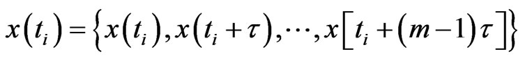 (1)
(1)
where,  is called the embedding dimension.
To construct a well-behaved phase space by delay time, a careful choice of  is critical. The delay time
  is commonly selected by using the autocorrelation

Figure 2. Daily discharge time series behaviour.

Figure 3. Autocorrelation of the original series.
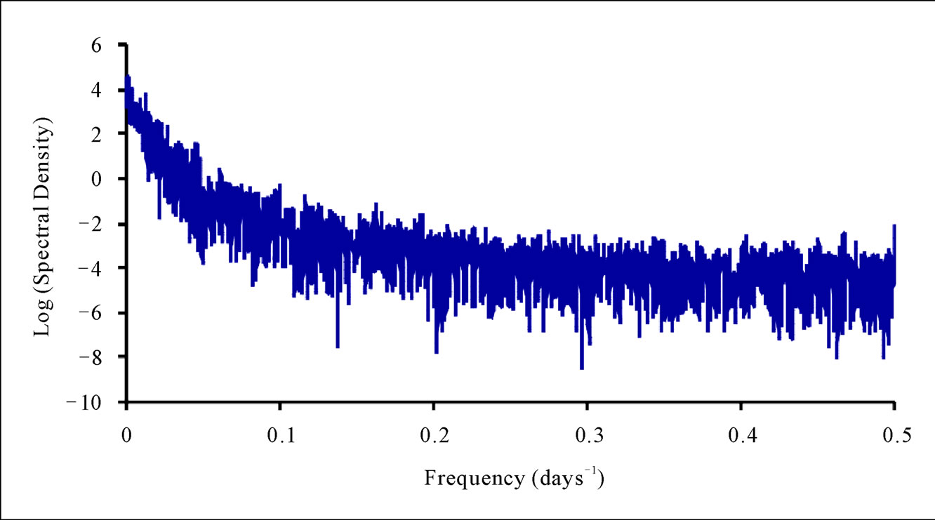
Figure 4. Spectral density of the filtered flow series (i.e., after the removal of annual periodicity).
function (ACF) method where ACF first attains zeros or drops below a small value, say , or the mutual information (MI) method according to Fraser and Swinney [14] where the MI attains a minimum. Here, the delay time
  was taken as the lag that first generates a zero autocorrelation, which is when the autocorrelation function crosses the zero line [15]. Figure 5 shows that this happened at lag time equals to 78 days. In practice, the estimate of
  is usually application and author dependent; for instance, some authors take the delay time as 1 day [2], 2 days [16], 7 days [17], 10 days [18], 20 days [19], 91 days [20], and 146 days [21]. These differences may arise from the nature of the autocorrelation function; to compare the influence of the delay time
  on the construction of state phase, the state phase maps can be plotted for differing
  values. The best
  value should make the state phase plot best unfolded. Towards this end, the state phase map was constructed for different
  values (
 = 1, 7, 10, 30, and 78). The best unfolding was obtained at
  = 78; therefore,
  = 78 was adopted for estimating the correlation dimension of the daily streamflow process.
Estimation of Correlation Dimension
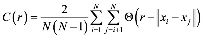
The most commonly used algorithm for computing the correlation dimension is the Grassberger-Procaccia algorithm [22]. For m-dimensional phase-space, the basic formula is given by
 (2)
(2)
subject to the constraints: 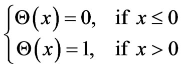
where,  is the Heaviside step function, and r is the radius between the pair of points in phase space. The straightforward estimator, Equation (2), is biased towards too small dimensions when the pairs entering the sum are statistically independent [23]. For time series data with nonzero autocorrelations, independence cannot be assumed; for instance, the embedding vectors at successive times are often also close in phase space due to the continuous time evolution [23], called temporal correlation. In the calculation of correlation dimension, temporal correlation may lead to serious underestimation unless the necessary care is taken.
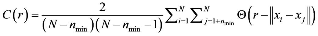
In order to avoid the problem of temporal correlation, a modified form of Equation (2) was used in the computation of the correlation dimension, as given by Equation (3) and implemented in the TISEAN 3.0 Software package.
 (3)
(3)

Figure 5. Detail of the autocorrelation for both original and the first differenced series.
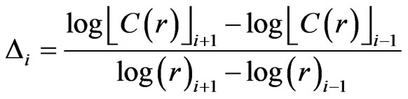
where, nmin is a threshold value such that pairs of vectors in the m-dimensional phase space which are closer in time than it are discarded to avoid temporal correlations that may contaminate the result. For the implementation of Equation (3), nmin was set to 182 for the daily flow series as suggested by Wang et al., [20]. The correlation integral C(r) and the correlation exponent D were computed for the data using different values of the delay time in order to examine objectively the appropriate delay time. For a finite data set, there is a radius below which there are no pairs of points, whereas at the other extreme, when the radius approaches the diameter of the cloud of points, the number of pairs will no longer increase as the radius increases (i.e., saturation point). The scaling region would be found somewhere between depopulation and saturation. Local slopes of “lnC(r)” versus “lnr” can indeed show clearly the scaling region if it does exist. The local slopes  for this case were computed according to Equation (4).
 (4)
(4)
2.3. Maximal Lyapunov Exponent
Since a positive maximal Lyapunov exponent is a strong signature of deterministic chaos, it is of considerable interest to determine its value; at least to complement the results obtained with the correlation dimension method. The first algorithm for this purpose was suggested by Wolf et al., [24]. This algorithm does not provide for the testing of the presence of exponential divergence, but just assumes its existence and thus yields a finite exponent for stochastic data also, where the true exponent is infinite [24]. For the computation of the maximal Lyapunov exponent, the algorithm introduced recently by Rosenstein et al., [25] and Kantz [26] independently was adopted. The implementation of the algorithm was done by using the TISEAN 3.0 Software package. The algorithm tests directly for the exponential divergence of nearby trajectories and thus allows one to decide whether it really makes sense to compute a Lyapunov exponent for a given data set. Essentially, the Lyapunov exponent is an average of these local divergence rates over the whole data.
2.4. Nonlinear Prediction
The use of chaotic models to forecast follows the recent trend of viewing most of the natural phenomena in a nonlinear way. In the chaotic approach, the governing assumption is that the discharges are driven by a multivariate dynamical system  and observed through the equation
  . Let m be the dimension of the attractor of the original and unobservable system
  ; the characteristics of the dynamics can be analyzed in a reconstructed phase space obtained by the d-dimensional vectors
  , where
  is called delay time and d, embedding dimension. As a consequence, in the reconstructed phase space there exists a deterministic dynamic f such that
 (5)
(5)
Equation (5) can be used to forecast the future of the time series  and a good prediction depends, essentially, on the ability of approximating the dynamic f with an estimate f. To execute nonlinear prediction as described above, there is the need to find an approximation of f in Equation (5). This can be done by several methods, starting with polynomial representations, from Kernel or Spline methods, up to Neural Networks, Wavelets or the Nearest Neighbours’ method. The nonlinear prediction was performed by adopting the method of local constant approximation using the Fast Neighbour search algorithm [23], and implemented in the TISEAN 3.0 Software package.
3. Results and Discussion
3.1. Correlation Dimension
Analyses of correlation dimension for the presence of deterministic chaos in streamflow series for timescales of daily, monthly and discharge derivative values show contrasting results. For instance, Savard [27] analysed the 27009 data point for Merced River discharge derivative  and found no low dimensional attractor, Wilcox et al., [19] presented a thorough CIA analysis of a standardised (periodicity removed), log-transformed runoff record and also found no low dimensional attractor, Wang et al., [20] carried out a similar detailed analysis on selected streamflow series in China, and found no low dimensional attractor; in general, their analysis revealed that using a short time lag results in a significant underestimate of the correlation dimension. However, Jayawardena and Lai [16] investigated rivers in Hong Kong, but used very short (2 - 3 days) time lags. Their reported correlation dimension of ~ 0.45 violate reality; no fewer than 3 degrees of freedom can generate chaos [21], and chaotic attractors cannot have a correlation dimension less than 1, except on a mapping [28]. Physically, a correlation dimension equals to 0.45 means that a river could arbitrarily jump from one location to another and likewise discontinuously vary its velocity and acceleration [28]. Against the backdrop of the assertions reported above, most of the results reported in literature on the fractal dimensions of hydrologic systems reveal inconsistent and unreliable applications of correlation integral analysis (CIA) in particular and chaos theory in general. To understand why records of daily river discharge are not likely to yield low dimensional attractors, it is useful to consider what happens to the data when it is embedded. Analysed as if they are random, river discharge data are most likely to fit the log-normal distribution, with most points falling in a narrow range of values and a few present as outliers.
The essence of the discussion above is to put the existing results in perspective so as to provide an objective framework for drawing conclusions on the findings in this study. It is important to note that some authors do not provide scaling region when reporting on the investigation aimed at determining the existence of chaos (e.g., [11,16,18]), whereas others do, but give no obvious scaling region (e.g., [2]). However, a clearly discernible scaling region is crucial for making a convincing and reliable estimate of correlation [23]. In respect of this, as reported in Figure 6, there is no visible scaling region; this does indicate that there is no presence of chaotic behaviour.
Looking at the result obtained further, given the limitations of the autocorrelation function approach, which was used here, an effort was made to study the effect of the delay time on the correlation dimension estimate. Figure 7 shows the relationship between the correlation exponent values and the embedding dimension while using differing values of delay time. It can be seen from Figures 7 and 8 that the correlation dimension exhibits an increasing behaviour without a saturation point, which is a basic indicator of deterministic chaos, thus suggesting the lack of the presence of chaos in the daily streamflow series. But Bellie, S. et al., [11], Havstad and Ehlers [29] contend that correlation dimension estimated with a considerably small or large delay time can result in underestimation and over-estimation of the correlation dimension. They opined that when the delay time is large, the successive coordinates in the embedding vector are independent of each other thus converging to a random process. This bring to mind the question of spurious correlation; most of these results do not take into account temporal correlation that might result when the Grassberger and Procaccia [22] formulation of the correlation integral equation is used directly without making allowance for the exclusion of temporal correlation. In addition, it is reported in some literatures that the first difference series of the streamflow gives important indications about the existence of a chaotic component (e.g., [2,30]). But as noted in Figure 9, it is obvious that both the filtered and original stream flow series do not show evidence of deterministic chaos. However though, one notable feature in Figure 9 is that when differenced data series was used, the correlation dimension is, in general, much larger than that of the original data, and does not converge at all. This finding accords with that of Provenzale et al., [31]; thus, one may be tempted to conclude that some of the results to the contrary, might be due to spurious convergence.
3.2. Maximal Lyapunov Exponent
For a time series generated by deterministic dynamical systems, positive characteristic exponents indicate the presence of chaos; this is why it is sufficient to calculate the largest Lyapunov exponent (λ). Table 1 reports the
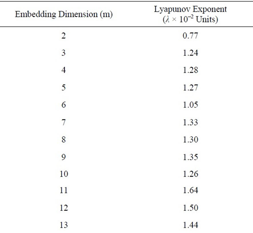
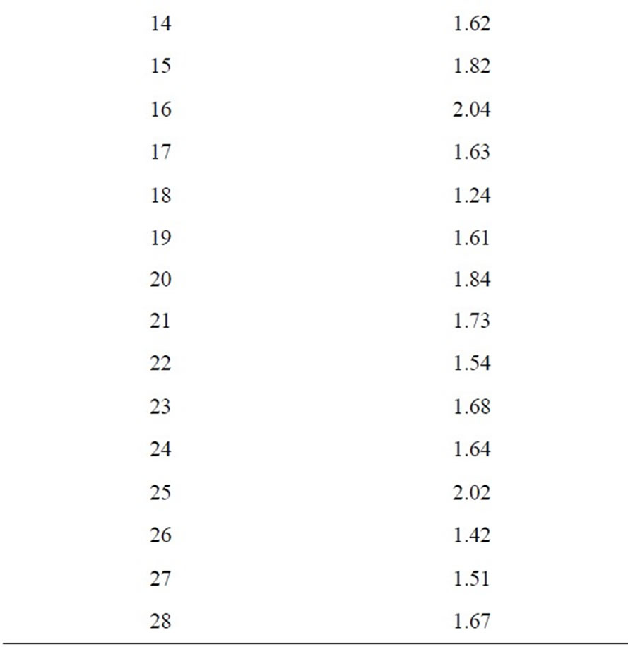
Table 1. Estimated maximal lyapunov exponent.
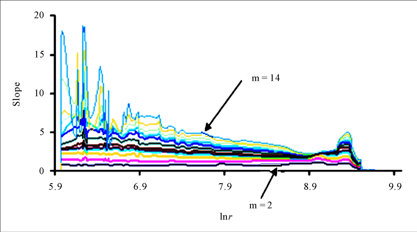
Figure 6. Correlation integral slopes for m between 2 and 14.
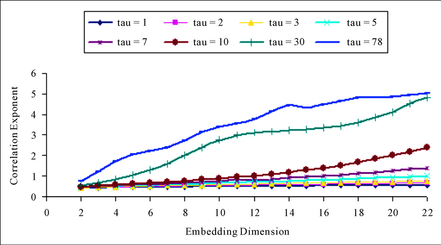
Figure 7. Correlation exponent versus embedding dimension for various delay time (tau) values.
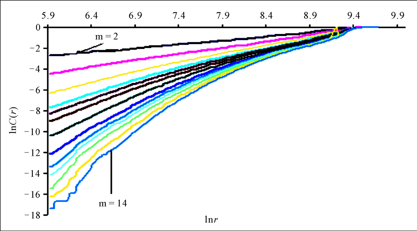
Figure 8. Correlation integrals for average daily discharge.
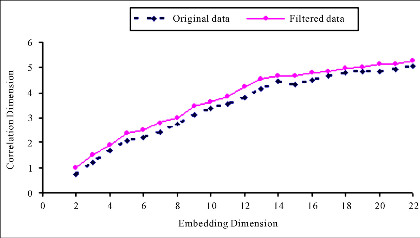
Figure 9. Relationship between correlation exponent and embedding dimension.
values of the Lyapunov exponent computed for the daily streamflow series. The values of λ reasonably are constant over a range of m between 3 and 28; based on the recommendation of Jayawardena and Lai [16], for this region where the values are constant, the mean of the series of λ generated in different dimensional phase-space: m = 3 to 28, was taken as the estimated maximal Lyapunov exponent. The resulting maximal Lyapunov exponent approximates λ = 0.01497 units, even if the convergence may not be completely satisfying, as typical in the presence of noise in the data series. The computed value is not distinctly larger than zero in any meaningful statistical sense, thus the maximal Lyapunov exponent λ as calculated here does not translate into an exhibition of deterministic chaos. Jayawardena and Lai [16] and Francesco and Villi [30] in their analysis respectively, reported the largest Lyapunov exponent for daily streamflow as 0.0086 and 0.007 units. These values are seemingly very low even though there are no currently available tests to determine if it is statistically greater than zero, but it does beg the question of whether daily flow series may actually be chaotic. Basically, their conclusions really contrast with that of Kember and Flower [32], who posited that daily river flows are unlikely to be chaotic.
3.3. Nonlinear Prediction
As reported in Casdagli [33], if the time series is chaotic, it is expected that the prediction errors will suddenly decrease to a value close to zero as the embedding dimension m is increased to the optimal dimension M, and remain close to zero for values of m greater than M; but if the time series is random, no such decrease should be observed. Figure 10 shows the prediction error (RMSE) against the embedding dimension. It is clear from this figure that this phenomenon is not exhibited here. This shows there is no discernible evidence of chaotic behaviour in the daily streamflow series. In the same context, for a chaotic time series, the correlation coefficient is close to 1 as m is increased to the optimal embedding dimension M and remains close to 1 for values of m above M [33]. But as reported in Figure 11, even though the correlation values remain close to 1 as m was increased to M (here, M = 3) and immediately afterwards, it does not remain constant when the embedding dimension was increased beyond the optimal embedding dimension, rather it decreased when the embedding dimension was increased. Though as suggested by Sugihara and May [34], this may be caused by contamination of nearby points in the high-dimensional embedding with points whose earlier coordinates (at low embedding dimensions) are close but whose recent coordinates (at high embedding dimensions) are distant. Therefore, it is probably difficult to proffer a plausible explanation for this. The situation may be analogous to periodic signal with additive noise, rather than chaotic signatures.
4. Conclusions
The study of the dynamics which controls the evolution of river flow, conducted in the light of chaos theory may have conflicting results. Some of these are more of a speculative character whereas others may have practical potentials. Following from the nonlinear analyses in this study, there is no discernible evidence to suggest the existence of low-dimensional chaos in the daily streamflow process of the Benue River. Though contradictory results abound on the existence of low-dimensional chaos in daily streamflows, it is paramount to note that
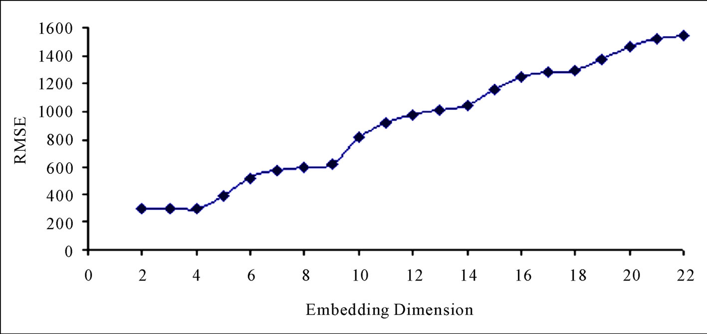
Figure 10. Relationship between degree of error (RMSE) and embedding dimension.
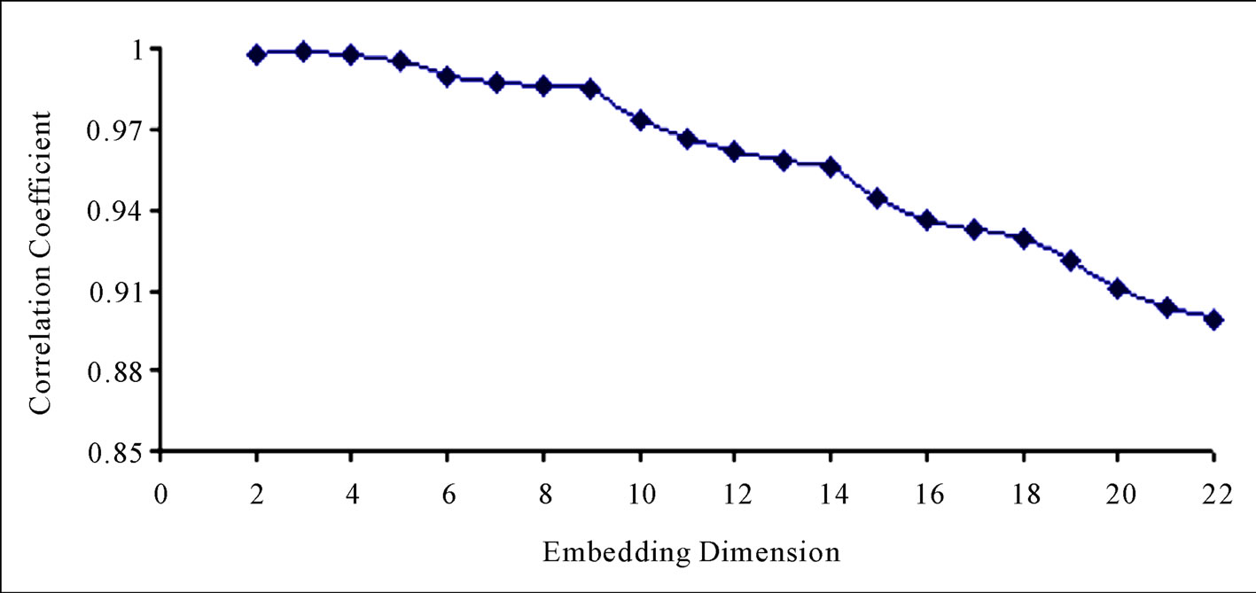
Figure 11. Relationship between correlation coefficient and embedding dimension.
since the dynamics of observed hydrological series is inevitably contaminated by not only measurement noise, but also dynamical noise, one may contend that the daily streamflow time series may span a wide dynamical range between deterministic chaos and periodic signal contaminated with additive noise. Added noise (measurement error) may strongly affect the nonlinear behaviour of deterministic system by decreasing the predictability, and invariably increases the dimension of an existing attractor. Thus, because streamflow process usually suffers from strong natural and anthropogenic disturbances which are themselves made up of both stochastic and deterministic components, it does beg the question of how a reliable identification of chaotic dynamics can be made even if the streamflow is actually low-dimensional. Considering also, for instance, the correlation dimension analysis provides information only on the number of variables influencing the dynamics of the system and does not in any plausible way identify the variables or the mathematical model for the dynamics of the river flow process. Hence, evidence of the existence of chaotic characteristics does not in any physical way, translate directly to determinism. However, regardless of the contradictory reports on the result of findings on deterministic chaos, this concept provides a profound technique for time series analysis and thus invariably allows for an intuitive understanding of dynamical systems.
REFERENCES
- B. Sivakumar, “Chaos Theory in Hydrology: Important Issues and Interpretations,” Journal of Hydrology, Vol. 227, No. 1-4, 2000, pp. 1-20. doi:10.1016/S0022-1694(99)00186-9
- P. Amilcare and L. Ridolfi, “Nonlinear Analysis of River Flow Time Series,” Water Resources Research, Vol. 33, No. 6, 1997, pp. 1353-1367. doi:10.1029/96WR03535
- P. Grassberger, “An Optimized Box-Assisted Algorithm for Fractal Dimensions,” Physical Review Letters A, Vol. 148, 1991, pp. 521-522.
- H. Inaoka and H. Takayasu, “Water Erosion as a Fractal Growth Process,” Physical Review E, Vol. 47, No. 2, 1993, pp. 899-910. doi:10.1103/PhysRevE.47.899
- S. D. Peckman, “New Results for Self-Similar Trees with Applications to River Networks,” Water Resources Research, Vol. 31, No. 4, 1995, pp. 1023-1029. doi:10.1029/94WR03155
- A. Rinaldo, G. K. Vogel, R. Rigon and I. RodriguezIturbe, “Can One Gauge the Shape of a Basin?” Water Resources Research, Vol. 31, No. 4, 1995, pp. 1119- 1127. doi:10.1029/94WR03290
- C. Nicolis and G. Nicolis, “Is There a Climatic Attractor?” Nature, Vol. 311, 1984, pp. 529-532. doi:10.1038/311529a0
- K. Fraedrich, “Estimating the Dimensions of Weather and Climate Attractors,” Journal of the Atmospheric Sciences, Vol. 43, No. 5, 1986, pp. 419-432. doi:10.1175/1520-0469(1986)043<0419:ETDOWA>2.0.CO;2
- K. Fraedrich, “Estimating Weather and Climate Predictability on Attractors,” Journal of the Atmospheric Sciences, Vol. 44, No. 4, 1987, pp. 722-728. doi:10.1175/1520-0469(1987)044<0722:EWACPO>2.0.CO;2
- P. Grassberger, “Do Climatic Attractors Exist?” Nature, Vol. 323, 1986, pp. 609-612. doi:10.1038/323609a0
- S. Bellie, L. Shie-Yui, L. Chih-Young and P. Kok-Kwang, “Singapore Rainfall Behaviour: Chaotic?” Journal of Hydrologic Engineering, Vol. 4, No. 1, 1999, pp. 38-48. doi:10.1061/(ASCE)1084-0699(1999)4:1(38)
- F. Takens, “Detecting Strange Attractors in Turbulence,” In: D. A. Rand and L. S. Young, Eds., Lecture Notes in Mathematics, Vol. 898, Springer-Verlag, New York, 1981, pp. 366-381.
- N. H. Packard, J. P. Crutchfield, J. D. Farmer and R. S. Shaw, “Geometry from a Time Series,” Physical Review Letters, Vol. 45, No. 9, 1980, pp. 712-716. doi:10.1103/PhysRevLett.45.712
- A. Fraser and H. L. Swinney, “Independent Coordinates for Strange Attractors from Mutual Information,” Physical Review A, Vol. 33, No. 2, 1986, pp. 1134-1140. doi:10.1103/PhysRevA.33.1134
- G. J. Mpitsos, H. C. Creech, C. S. Cohan and M. Mendelson, “Variability and Chaos: Neuron-Integrative Principles in Self-Organization of Motor Patterns,” In: B.-L. Hao, Ed., Directions in Chaos, Vol. 1, 1987, World Scientific, pp. 162-190.
- A. W. Jayawardena and F. Lai, “Analysis and Prediction of Chaos in Rainfall and Streamflow Time Series,” Journal of Hydrology, Vol. 153, No. 1-4, 1994, pp. 23-52. doi:10.1016/0022-1694(94)90185-6
- M. N. Islam and B. Sivakumar, “Characterization and Prediction of Runoff Dynamics: A Nonlinear Dynamical View,” Advances in Water Resources, Vol. 25, No. 2, 2002, pp. 179-190. doi:10.1016/S0309-1708(01)00053-7
- A. Elshorbagy, S. P. Simonovic and U. S. Panu, “Estimation of Missing Streamflow Data Using Principles of Chaos Theory,” Journal of Hydrology, Vol. 255, 2002, pp. 125-133. doi:10.1016/S0022-1694(01)00513-3
- B. P. Wilcox, M. S. Seyfried and T. H. Matison, “Searching for Chaotic Dynamics in Snowmelt Runoff,” Water Resources Research, Vol. 27, No. 6, 1991, pp. 1005-1010.
- W. Wang, P. H. A. J. M. Van Gelder and J. K. Vrijing; “Detection of Changes in Streamflow Series in Western Europe over 1901-2000,” Water Science and Technology, Water Supply, Vol. 5, No. 6, 2005, pp. 289-299.
- G. B. Pasternack, “Does the River Run Wild? Assessing Chaos in Hydrological Systems,” Advances in Water Resources, Vol. 23, No. 3, 1999, pp. 253-260. doi:10.1016/S0309-1708(99)00008-1
- P. Grassberger and I. Procaccia, “Measuring the Strangeness of Strange Attractors,” Physica D, Vol. 9, No. 1-2, 1983, pp. 189-208. doi:10.1016/0167-2789(83)90298-1
- K. Holger and T. Schreiber, “Nonlinear Time Series Analysis,” Cambridge University Press, Cambridge, 1997, pp. 42-86.
- A. Wolf, J. B. Swift, H. L. Swinney and J. A. Vastano, “Determining Lyapunov Exponents from a Time Series,” Physica D, Vol. 16, No. 3, 1985, pp. 285-317. doi:10.1016/0167-2789(85)90011-9
- M. T. Rosenstein, J. J. Collins and C. J. De Luca, “A Practical Method for Calculating Largest Lyapunov Exponents for Small Data Sets,” Physica D, Vol. 65, 1993, pp. 117-134. doi:10.1016/0167-2789(93)90009-P
- H. Kantz, “A Robust Method to Estimate the Maximal Lyapunov Exponent of a Time Series,” Physical Letters A, Vol. 185, No. 1, 1994, pp. 77-87. doi:10.1016/0375-9601(94)90991-1
- C. S. Savard, “Looking for Chaos in Streamflow with Discharge Derivative Data,” EOS Transactions AGU (Spring Meeting Supplement), Vol. 73, No. 14, 1992, p. 50.
- E. Ott, “Chaos in Dynamical Systems,” Cambridge University Press, New York, 1993.
- J. W. Havstad and G. Mayer-Kress, “Attractor Dimension of Non-Stationary Dynamical Systems from Small Data Sets,” Physical Review A, Vol. 39, No. 2, 1989, pp. 845- 853. doi:10.1103/PhysRevA.39.845
- L. Francesco and V. Villi, “Chaotic Forecasting of Discharge Time Series: A Case Study,” Journal of the American Water Resources Association, Vol. 87, No. 2, 2001, pp. 271-279.
- A. Provenzale, A. Smith, R. Vio and G. Murante, “Distinguishing between Low Dimensional Dynamics and Randomness in Measured Time Series,” Physica D, Vol. 58, No. 1, 1992, pp. 31-49. doi:10.1016/0167-2789(92)90100-2
- G. Kember and A. C. Flower, “Forecasting River Flow Using Nonlinear Dynamics,” Stochastic Hydrology and Hydraulics, Vol. 7, 1993, pp. 205-212. doi:10.1007/BF01585599
- M. Casdagli, “Nonlinear Prediction of Chaotic Time Series,” Physica D, Vol. 35, 1989, pp. 335-356. doi:10.1016/0167-2789(89)90074-2
- G. Sugihara and R. M. May, “Nonlinear Forecasting as a Way of Distinguishing Chaos from Measurement Error in Time Series,” Nature, Vol. 344, 1990, pp. 734-741. doi:10.1038/344734a0