Journal of Software Engineering and Applications
Vol.6 No.4A(2013), Article ID:30427,13 pages DOI:10.4236/jsea.2013.64A006
Aperiodic Checkpoint Placement Algorithms—Survey and Comparison*
![]()
Department of Information Engineering, Hiroshima University, Hiroshima, Japan.
Email: dohi@rel.hiroshima-u.ac.jp, okamu@rel.hiroshima-u.ac.jp
Copyright © 2013 Shunsuke Hiroyama et al. This is an open access article distributed under the Creative Commons Attribution License, which permits unrestricted use, distribution, and reproduction in any medium, provided the original work is properly cited.
Received January 23rd, 2013; revised February 24th, 2013; accepted March 4th, 2013
Keywords: Checkpoint Placement; Aperiodic Policy; Availability Models; Computation Algorithms; Comparison
ABSTRACT
In this article we summarize some aperiodic checkpoint placement algorithms for a software system over infinite and finite operation time horizons, and compare them in terms of computational accuracy. The underlying problem is formulated as the maximization of steady-state system availability and is to determine the optimal aperiodic checkpoint sequence. We present two exact computation algorithms in both forward and backward manners and two approximate ones; constant hazard approximation and fluid approximation, toward this end. In numerical examples with Weibull system failure time distribution, it is shown that the combined algorithm with the fluid approximation can calculate effectively the exact solutions on the optimal aperiodic checkpoint sequence.
1. Introduction
It is well known that the system failure in large-scale computer systems can lead to a huge economic or critical social loss. Checkpointing and rollback recovery is a commonly used technique for improving the reliability/availability of fault-tolerant computing systems, and is regarded as a low-cost software dependability technique from the standpoint of environment diversity. Especially, when file systems to write and/or read data are designed, checkpoint (CP) generations back up periodically/aperiodically the significant data on a primary medium to safe secondary media, and play a significant role to limit the amount of data processing for recovery actions after system failures occur. If CPs are frequently taken, a larger overhead will be incurred. Conversely, if only a few CPs are taken, a larger overhead after a system failure will be required in rollback recovery actions. Hence, it is important to determine the optimal CP sequence taking account of the trade-off between two kinds of overhead factor above. In many cases, the system failure phenomenon is described with a probability distribution called the system-failure time distribution, and the optimal CP sequence is determined based on any stochastic model. For the excellent survey on this topic, see [2,3].
First Young [4] obtains the optimal CP interval approximately for a computation restart after system failures. Baccelli [5], Chandy et al. [6,7], Dohi et al. [8-10], Gelenbe and Derochette [11], Gelenbe [12], Gelenbe and Hernandez [13], Goes and Sumita [14], Goes [15], Grassi et al. [16], Kobayashi and Dohi [17], Kulkarni et al. [18], Nicola and van Spanje [19], Sumita et al. [20], among others, propose performance evaluation models for database recovery, and calculate the optimal CP intervals which maximize the system availability or minimize the mean overhead during the normal operation. L’Ecuyer and Malenfant [21] formulate a dynamic CP placement problem by a Markov decision process. Ziv and Bruck [22] analyze an online algorithm for a probabilistic CP placement. Vaidya [23] examines an impact of checkpoint latency on overhead ratio for a simple CP model. Okamura et al. [24] reformulate the Vaidya model [23] with a semi-Markov decision process and further develop a reinforcement adaptive learning algorithm for CP placement. For several CP models in the literature, the periodic CP intervals are implicitly assumed. This is because the periodic CP intervals maximize the steadystate system availability, and in many cases, are better than the randomized CP ones which are given by independent and identically distributed random variables. However, it is worth noting that the periodic CP strategies can not be always validated in some cases and less performe than the aperiodic CP placement. In general, it is known that the way to place the optimal CP sequence strongly depends on both kind of objective functions (system availability, mean overhead, etc.) and kind of system-failure time distribution. Since the aperiodic CP involves the periodic CP as a special case, it is meaningful to consider the aperiodic CP placement algorithm for file systems.
When the system-failure time obeys a non-exponential distribution, it is easily shown that the aperiodic CP placement is not worse than the periodic CP one. Toueg and Babao lu [25] develop a dynamic programming (DP) algorithm which minimizes expected execution time of tasks placing CPs between two consecutive tasks under very general assumptions. Kaio and Osaki [26] consider an approximate aperiodic CP placement algorithm under the asssumption that the conditional system-failure probability is constant during the successive CPs. Fukumoto et al. [27,28] and Ling et al. [29] propose fluid approximation methods based on a variational calculus approach to derive the cost-optimal aperiodic CP sequence. Ozaki et al. [30,31] give an exact aperiodic CP placement algorithm and further develop an estimation scheme under the incomplete knowledge on systemfailure time distribution. In a fashion similar to the above approach, Dohi et al. [32] formulate another aperiodic CP placement problem with equality constraints. Iwamoto et al. [33], Okamura et al. [34,35], and Okamura and Dohi [36] propose different DP-based algorithms from Toueg and Babao
 lu [25] under the availability criterion, by taking account of another dependability technique, called the software rejuvenation in the presense of software aging, where the system failure caused by the aging is not exponentially distributed. Recently, Ozaki et al. [37] propose a fixed-point type algorithm for an aperiodic CP placement with an infinite operation-time horizon. In this way, considerable attentions have been paid for aperiodic CP placement problems in past.
Nevertheless, it can be pointed out that no effective aperiodic CP placement algorithm has been known yet when the number of CPs is very large. The constant hazard approximation [26] and fluid approximation [27-29] may poorly work in such a case. The search-based iteration algorithm in [30,31] and the DP-based algorithm in [33-36], which are regarded as exact computation algorithms, also require the very careful adjustment to determine the number of CPs if the operation time for a file system is finite. As the operation time becomes longer, in general, the number of CPs is sensitive to not only the determination of the aperiodic CP sequence but also the resulting dependability measures. In this article we summarize some aperiodic CP placement algorithms for a software system over infinite and finite operationtime horizons, and compare them in terms of computational accuracy. It is proposed to combine the fluid approximation with an exact computation algorithm in determining the initial value of the number of CPs. The idea is quite simple, but we show that the combined algorithm with the fluid approximation can calculate effectively the exact solutions on the optimal aperiodic CP sequence.
2. Formulation of Optimal CP Placement
First, consider a centralized file system with sequential checkpoint (CP) over an infinite time horizon. The system operation starts at time , and the CP is sequentially placed at time
  to back up the data processed in the file system. At each CP,
  , all the file data on the main memory is saved to a safe secondary medium, where the fixed cost (time overhead)
  is needed per each CP placement. It is assumed that the system operation stops during the checkpointing, so during the period
  the file system does not deteriorate. System failure may occur according to an absolutely continuous and non-decreasing probability distribution function
  having density function
  and finite mean
 . Upon a system failure, a rollback recovery takes place immediately where the file data saved at the last CP creation is used. Next, a CP restart is performed and the file data is recovered to the state just before the system failure occurs. The time length required for the CP restart is given by the function
 , which depends on the system failure time, and is assumed to be differentiable and increasing. We call the function
  the recovery function in this article. After the completion of CP restart, an additional CP must be created to save the current state and the system operation restarts with the same condition as the initial point of time
 . The similar cycle repeats again and again over an infinite time horizon.
The problem is to determine the optimal CP sequence  maximizing the steady-state system availability:
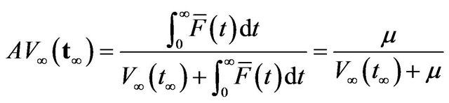 (1)
(1)
where
and
 (2)
(2)
denotes the expected operaing cost with . It is evident that the underlying problem is reduced to a simple minimization problem
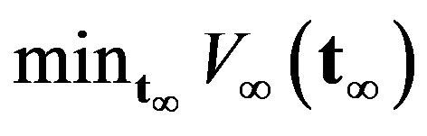 . In this problem, the expected recovery cost is usually given by the affine form

for the system failure time , where
  and
and  are given constants. Instead, by replacing the above CP cost and recovery cost by
  and
and
 , this is equivallent to the classical inspection problem by Barlow and Proschan [38]. Figure 1 illustrates the configuration of the underlying CP placement with a finite operation-time horizon
 .
.
From the analogy to the inspection problem, it can be easily shown that the optimal CP sequence
 maximizing the steady-state system availability is a non-increasing sequence under the assumption that the system failure time distribution
  is PF2 (Polya Frequency Function of Order 2) [38], if there exists the optimal CP sequence
  satisfying
 . Then, it must satisfy the following first order condition of optimality:
 (3)
(3)
From the condition of optimality, an algorithm to derive the optimal CP sequence  which minimezes
  or equivalentlly maximizes
  can be derived as follows.
Forward CP Placement Algorithm for an Infinite Operation-Time Horizon: [30,31,37].
Step 1: Set  satisfying
 .
.
Step 2: Compute  using Equation (3).
Step 3: For  -th CP
 , if
, if  , then decrease
  and Go to Step 2.
Step 4: For  -th CP
 , if
, if , then increase
  and Go to Step 2.
Step 5: For the resulting CP sequence , if
, if , then Stop the procedure, where
  is sufficiently small tolerance value and
 .
.
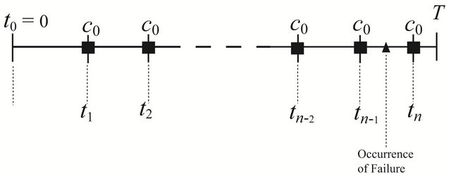
Figure 1. Configuration of the aperiodic CP placement with a finite operation-time horizon T.
In the above algorithm, arbitrary increasing and decreasing operations in Steps 3 and 4 can be taken to speed up the computation. The simplest method would be the bisection serach method. As the simplest case, if the system failure time is given by the exponential distribution with mean , it is well known that the optimal CP sequence is periodic, i.e.,
 .
.
Since the processing time for a given transaction is in general bounded, the CP placement for an infinite-time horizon may be questionable in many practical applications. As a natural extension of the infinite-time horizon problem, it would be interesting to consider the finite operation-time horizon problem, because  is a special case. Suppose that the time horizon of operation for the file system is finite, say,
  , which can be regarded as a fixed transaction processing time. For a finite sequence
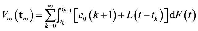
 , the expected operating cost is given by
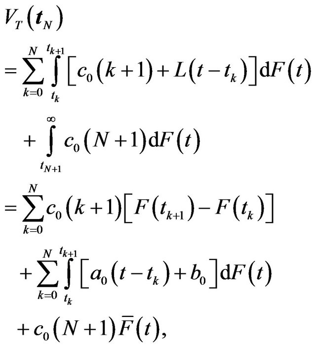 (4)
(4)
where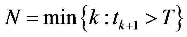 . Also we suppose that the file system restarts with a fixed CP overhead
  just after the time
![]() , if the system failure does not occur. Since the steady-state system availability is given by
, if the system failure does not occur. Since the steady-state system availability is given by
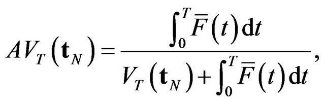 (5)
(5)
the underlying maximization problem reduces to . It should be noted that the recovery cost does not occur at
 . To simplify the notation, we define
  in this article. When the recocery cost function is the affine form i.e.,
  , differentiating Equation (4) with respect to
  and setting it equal to 0 yield Equation (3) again for
 and a given
 .
.
Since the finite operation-time horizon problem involves the constraint  on the number of CPs, it is impossible to apply directly the forward CP placement algorithm for an infinite operation-time horizon problem. However, by adjusting the value of
 , we can develop the similar algorithm to compute the optimal CP sequence. The basic idea is to utilize the non-increasing property of CP sequence under the PF2 assumption for an arbitrary number
 . Based on the result for an infinite time horizon [30,31,37], we modify the forward CP placement algorithm as follows.
Forward CP Placement Algorithm for a Finite Operation-Time Horizon: [30,31].
Step 1: Set the lower and upper bounds of  by
by  and
and , respectively.
Step 2: .
.
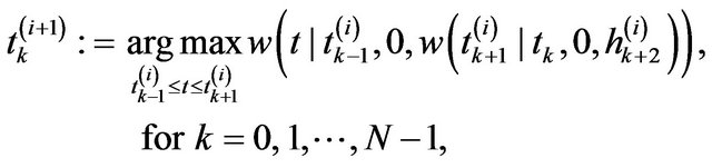
Step 3: For , compute the CP sequence
  by
by

Step 4: For ,
,
Step 4.1: If , then
  and Go to Step 2.
Step 4.2: If , then
  and Go to Step 2.
Step 5: For an arbitrary tolerance level , if
, if  , then
  and Go to Step 2.
Step 6: For an arbitrary tolerance level , if
, if  , then
  and Go to Step 2.
Step 7: End.
For all possible combinations of , we calculate all expected operating costs using the above algorithm, and determine both the optimal number of CPs,
  and its associated CP sequence
 . It should be noted that the above two algorithms can be validated only when the system failure time distribution is PF2 and the resulting CP sequence is non-increasing, i.e.,
 . The most significant point is that these algorithms are very fast to derive the optimal CP sequence, but strongly depend on the initial value
 . In the worst case, it is evident that these algorithms are sometime unstable and that the resulting CP sequence may not converge to the optimal solution. To overcome this point, the careful selection of the initial value
  is essentially needed, so we improve it by the following algorithm.
Improved Forward CP Placement Algorithm for a Finite Operation-Time Horizon:
Step 1: Set ,
,  ,
,  and the upper bound of serach range
 .
.
Step 2: Set  and
and .
.
Step 2.1: .
.
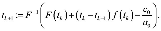
Step 2.2: For , compute
  satisfying
Step 2.3: Compute the corresponding expected operating cost and set it as  based on
 .
.
Step 2.4: If , then
  and
and , and Go to Step 3, otherwise
  and Go to Step 2.1, where
 .
.
Step 3: If  and
and , then
  and Go to Step 2, otherwise Go to Step.
Step 4: For all , search the minimum value
  and its associated CP sequence
 .
.
Since the initial value  in the above algorithm can be adjusted gradually from 0, the stability for the original forward CP placement algorithm could be rather improved. However, when
  is relatively large, the solution may still drop in the local minimum, and even the improved algorithm may fail to converge. In our numerical experiments, even when
 , the search of the initial value
  was sometimes unsuccsessful. In addition, it can be obvious that the computation cost of the improved algorithm is much larger than the original forward CP placement algorithm. In the following section, we introduce more stable algorithm on computation.
3. Backward CP Placement Algorithm
For the same aperiodic CP placement problem, Naruse et al. [39,40] propose to solve the optimality condition in the backward manner. Letting  for a given
 , the optimal CP sequence
  has to satisfy the first ortder condition
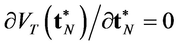 , and should be the solution of the following
  simultaneous equations:
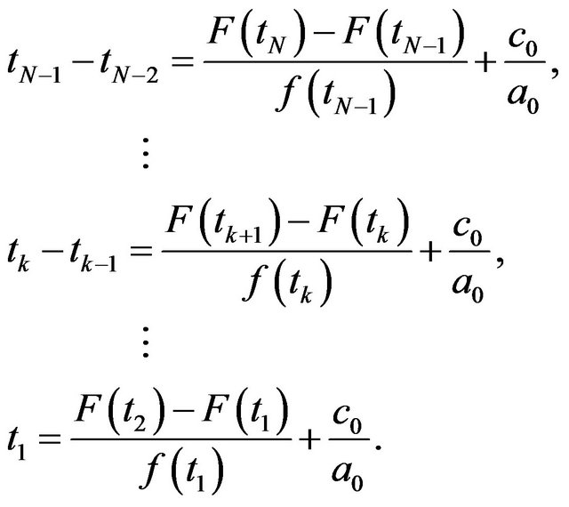 (6)
(6)
Although this algorithm does not depend on the PF2 property, it is not feasible for a large number of CPs, because an explosion of the number of simultaneous equations occurs for increasing the number of CPs. In fact, the authors in [40] present only a toy problem with a very small number of CPs.
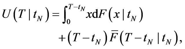
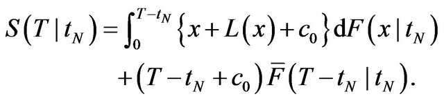
The most realistic backward algorithm is already given by Iwamoto et al. [33], and is based on the well-known dynamic programing (DP). Since this algorithm does not also depend on the PF2 property, it is applicable even to the more general failure time distribution. During the time period between two successive CPs,
 the expected operation time
  and the mean time length of one cycle
  are given by
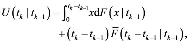 (7)
(7)
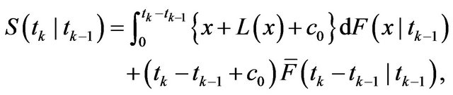 (8)
(8)
respectively, where one cycle is defined as the time interval between two successive renewal points. In Equations (7) and (8),  represents the conditional probability distribution:
 (9)
(9)
At the end of the operation-time , the above expressions are rewritten as follows.
 (10)
(10)
 (11)
(11)
From the principle of optimality, we obtain the following DP equations:
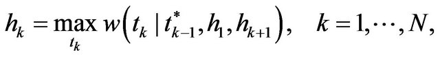 (12)
(12)
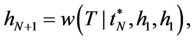 (13)
(13)
where the function  is given by
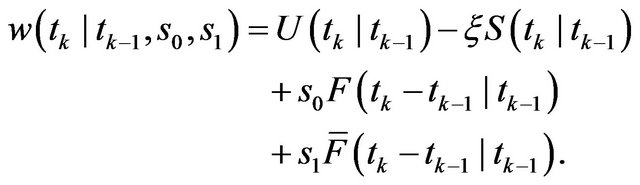 (14)
(14)
In the above equation,  indicates the maximum steady-state system availability and
 ,
,  , are relative value functions in the DP. The derivation of the optimal CP intervals is equivalent to finding
  which satisfy the DP equations. Following Iwamoto et al. [33], we apply the policy iteration algorithm which is effective to solve the above type of functional equations. Instead of the original function
 , define for convenience the following function:
 (15)
(15)
Then the DP-based CP placement algorithm is given in the following:
Backward CP Placement Algorithm: [33].
Step 1: Give initial values
 (16)
(16)
 (17)
(17)
 (18)
(18)
where  is the iteration number.
Step 2: Compute  under the policy
 .
.
Step 3: Solve the following optimization problems:
 (19)
(19)
 (20)
(20)
Step 4: For all , if
, if , stop the algorithm, where
 ![]() is an error tolerance, otherwise, let
is an error tolerance, otherwise, let  and go to Step 2.
In Step 2 of the above algorithm, we have to calculate the relative value functions. From the original DP Equations (12) and (13), we find that the relative value functions under a fixed policy  must satisfy the following linear equation:
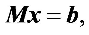 (21)
(21)
where
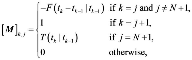 (22)
(22)
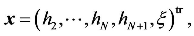 (23)
(23)
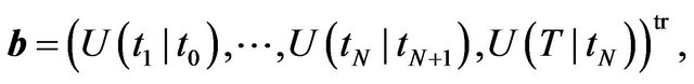 (24)
(24)
 denotes the
  -element of matrix, and
  represents transpose of vector. Without a loss of generality, we set
  in the above algorithm.
For both forward and backward CP placement algorithms, it is essential to determine the number of CPs,  , during the finite operation-time horizon. In other words, if the initial value of
  in the algorithms can be known in advance, it can be easily explored with any low-cost search technique. In the following section, we introduce two approximate algorithms for the finite operation-time horizon problem.
4. Approximate CP Placement Algorithms
4.1. Constant Hazard Approximation
If the time interval between two successive CPs,  , is sufficiently short, the system-failure probability during the time interval can be approximately considered as a constant, i.e.,
 (25)
(25)
Kaio and Osaki [26] approximate the expected operating cost,  as a function of
 ![]() under the above assumption. Here we derive the same result as [26] in a different way. Let
under the above assumption. Here we derive the same result as [26] in a different way. Let  be the system-failure time having the probability distribution
 . For an arbitrary probability
 , define the CP sequence satisfying the following quantile condition:
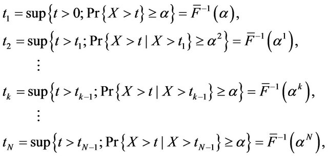
where 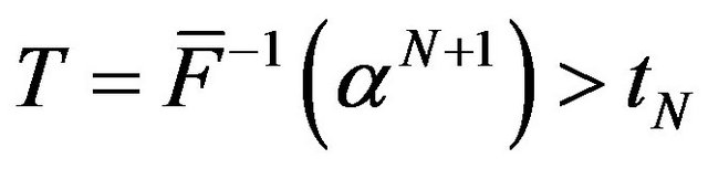 and
and . From a few algebraic manipulations, the expected operating cost can be represented as a function of
 ![]() as
as
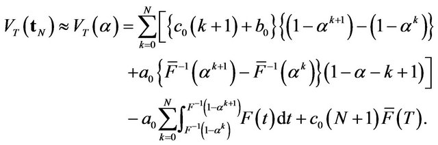 (26)
(26)
By minimizing the expected operating cost with respect to ![]() and substituting the optimal
and substituting the optimal ![]() into
into , an aperiodic CP sequence is approximately derived. For this approximate algorithm, we need to determine the number of CPs in advance. Also, even though the exact number of CPs is known, the approximate algorithm does not guarantee an exactly optimal CP sequence.
4.2. Fluid Approximation
The next approximate algorithm focuses on the determination of the number of CPs. Let  be the average frequency of CP placement at time instant
 . Then the time interval between two succsessive CPs at time
  is approximately given by
 . Using
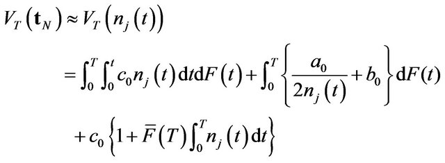
 , the expected operating cost over an infinite operation-time horizon is approximately expressed as a functional of
 :
:
 (27)
(27)
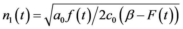
Then, the optimization problem with an infiniteoperation time horizon reduces to a variational culculus![]() . By solving the corresponding Euler equation, we have the optimal CP frequency
. By solving the corresponding Euler equation, we have the optimal CP frequency
![]() .
.
On the other hand, in the case with a large operation-time horizon, Ozaki et al. [30,31] assume that the probability of the occurrence of a system failure can be negligible even if the file system survives after the time horizon, and derive the average frequency of CP placement by
 where the control parameter
  is determined so as to satisfy
 . Naruse et al. [40] also propose a modified average frequency of CP placement by
 where
where
 (28)
(28)
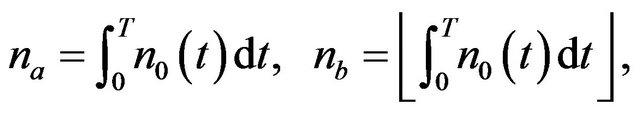
and  is the integer part satisfying
 .
.
Hence, the optimal aperiodic CP sequence is determined by  or
or 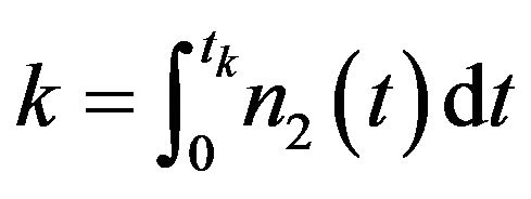 for
for
 . Substituting the approximate CP sequence yields the following approximate expected operating cost:
 (29)
(29)
for . As mentioned before, both two approximate algorithms do not also guarantee an exactly optimal CP sequence. However, it is worth mentioning that
  in Equation (28) provides a very near value of the exact number of CPs. By setting
  as the initial value of
  in the forward or backward CP placement algorithm and adjusting its integer value via a simple bisection method, we can seek the number of CPs placed up to the finite operation time
![]() .
.
The main difference between the constant hazard approximation and the fluid approximation is that the latter is based on the number of CPs by
 where
where . For a given
 ![]() and
and , both forward and backward algorithms are applicable. By combining the fluid approximation with the forward or backward CP placement algorithm, it is possible to speed up the computation to calcurate the optimal CP sequense.
5. Numerical Examples
We calculate numerically the optimal CP sequence and the corresponding steady-state system availability. Suppose that the failure time distribution obeys the Weibull distribution:
 (30)
(30)
with shape parameter  and scale parameter
 . In this case, the failure (hazard) rate
  and the inverse function
  in the algorithms are given by
 (31)
(31)
 (32)
(32)
For the operation-time horizon , we calculate the optimal CP sequence with an exact solution algorithm (forward or backward CP placement algorithm) and two approximate algorithms, and derive both the number of CPs and the steady-state system availability. When
 , it is noted that the system failure time distribution is strictly DFR (Decreasing Failure Rate) and is not PF2. Hence we apply only the backward CP placement algorithm for this case. In the case with PF2, two exact solution algorithms provide the exactly same results, where the number of CPs is adjusted from the initial value
  given in Equation (28). For the other model parameters, we set
 ,
,  and
and .
.
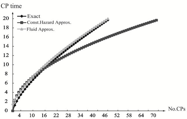
Figure 2 depicts the optimal CP time sequence with different shape parameter  for
for  and
and , in the strict DFR case (a) with
 , the optimal CP time behaves as convex functions with respect to the number of CPs for both exact and approximate methods. It can be seen that the two approximate methods poorly work except around 14-th CP. In the CFR (Constant Failure Rate) case (b) with
 , the optimal CP time becomes a linear function, so all the methods give the almost same periodic CP time sequence. In the strict IFR (Increasing Failure Rate) case (c) with
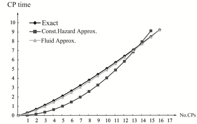
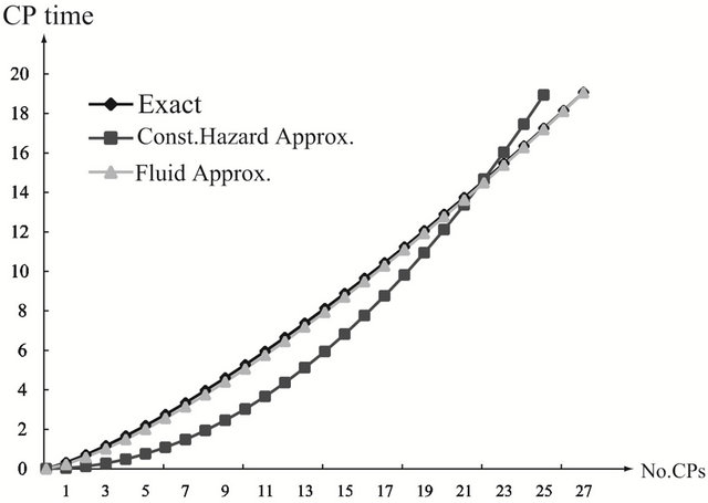
 , the optimal CP time shows concave functions of the number of CPs, and two approximate methods provide rather close values to the exact solution. In Figures 3 and 4, we show the optimal CP time sequence with
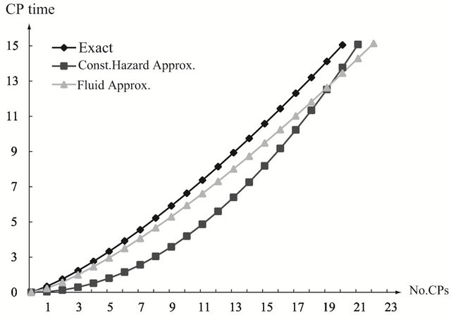
  and
and . As the finite operation time becomes longer, the constant hazard approximation tends to be far from the exact solution, when the system failure time distribution is strict IFR. On the other hand, the fluid approximation gives the almost similar CP time sequence to the exact solution. However, in Figure 3(a), the fluid approximation takes a bit differnt value of the optimal CP time sequence from the exact solution. In
 (a)
(a)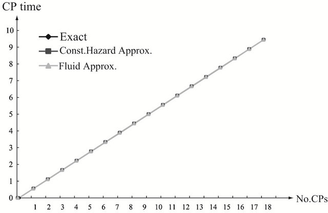 (b)
(b)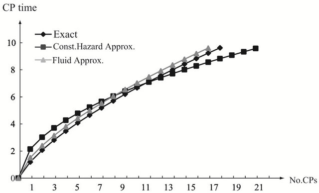 (c)
(c)
Figure 2. Aperiodic CP placement with different shape parameters for T = 10. (a) Case 1: γ = 0.5 and θ = 10; (b) Case 2: γ = 1.0 and θ = 10; (c) Case 3: γ = 2.0 and θ = 10.
other words, the computation accuracy for two approximate algorithms becomes worse as the shape parameter deviates from  more and more. In Figure 5, we investgate the dependence of the optimal aperiodic CP time on the scale parametr and the operation time in the strict IFR case. Looking at (a) to (f), only the constant hazard approximation shows the different behavior from the exact solutions.
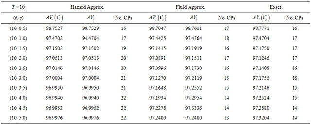
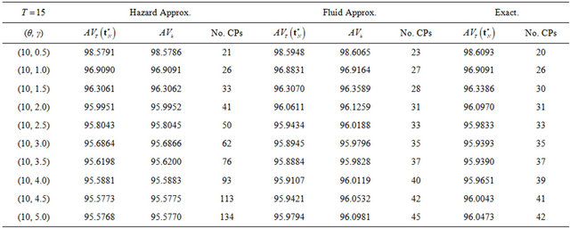
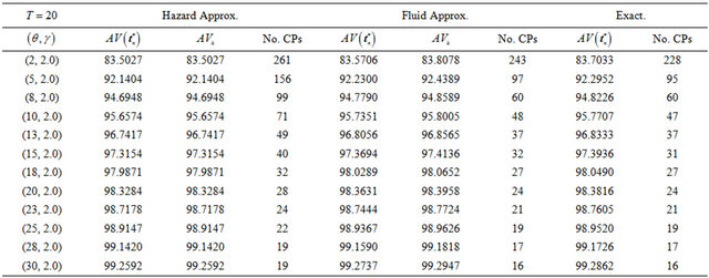
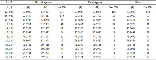
Next, we compare two approximation methods with the exact computation in terms of steady-state system availability more precisely. In Table 1, we present the steady-state system availability and the number of CPs
 (a)
(a)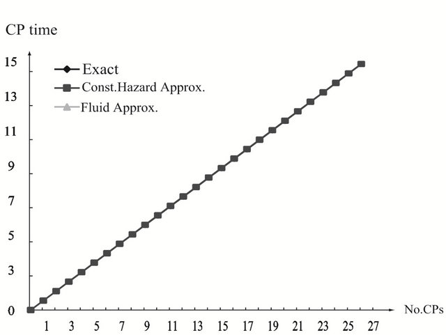 (b)
(b)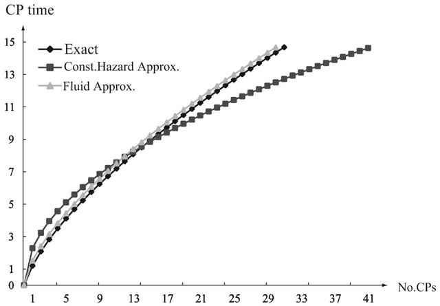 (c)
(c)
Figure 3. Aperiodic CP placement with different shape parameters for T = 15. (a) Case 1: γ = 0.5 and θ = 10; (b) Case 2: γ = 1.0 and θ = 10; (c) Case 3: γ = 2.0 and θ = 10.
for varying the failure parameters  when three algorithms are used. In the terms of approximate algorithms,
  is caluculated by substituting each approximate CP sequence into Equation (5), so that
  and
and  in Equations (26) and (29)
are calculated, where  is used for the
 (a)
(a)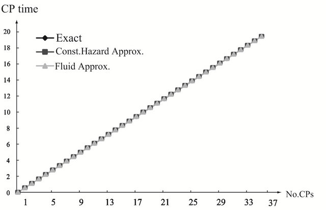 (b)
(b) (c)
(c)
Figure 4. Aperiodic CP placement with different shape parameters for T = 20. (a) Case 1: γ = 0.5 and θ = 10; (b) Case 2: γ = 1.0 and θ = 10; (c) Case 3: γ = 2.0 and θ = 10.
fluid approximation. Tables 1 and 2 present the dependence of the shape and the scale parameters on the steady-state system availability, respectively. When  increases, then the system tends to fail as the operation time goes on, and the system availability does not always decrease in Table 1. In this case, the number of CPs does not always increase from Table 1. When
  increases, then the mean time to system failure (MTTSF) also increases and the steady-state system availability is
Table 1. Dependence of the shape parameter γ on the steady-state system availability. (a) Case 1: T = 10; (b) Case 2: T = 15; (c) Case 3: T = 20.
(a)
(b)
(c)
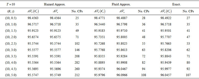
Table 2. Dependence of the scale parameter  on the steady-state system availability. (a) Case 1: T = 10; (b) Case 2: T = 15; (c) Case 3: T = 20.
(a)
(b)
(c)
 (a)
(a)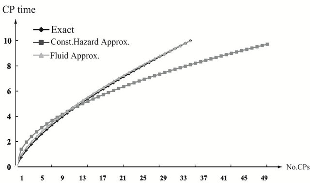 (b)
(b)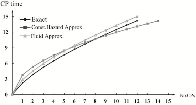 (c)
(c) (d)
(d)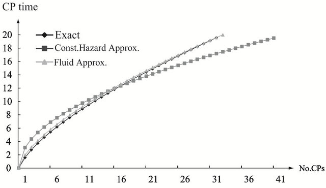 (e)
(e)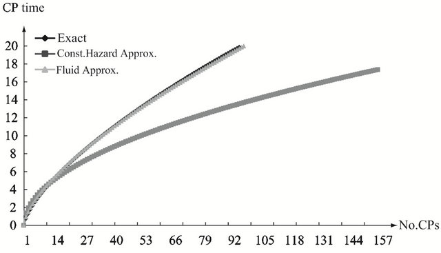 (f)
(f)
Figure 5. Aperiodic CP placement with different scale parameters and operation time for γ = 2.0. (a) Case 1: θ = 5 and T = 10; (b) Case 2: θ = 20 and T = 10; (c) Case 3: θ = 5 and T = 15; (d) Case 4: θ = 25 and T = 15; (e) Case 5: θ = 5 and T = 20; (f) Case 6: θ = 20 and T = 20.
expected to increse.This intuitive observation as well as the decreasing trend of the number of CPs are corect from Table 2. If we compare the minimum steady-state system availability calculated by the exact solution algorithm with the other ones, the relative error in both approximate methods can be found at the order of . Especially, the reason why the constant hazard approximation works well is that it increases the number of CPs so as to increase the system availability. This implies that even the constant hazard approximation probvides the nice approximate performance on the maximum system availability. On the other hand, the number of CPs in the fluid approximation is also close to the exact one. Through these numerical examples, it can be concluded that if the steady-state system availability is evaluated with higher accuracy such as four or five nines, it is needed to apply the exact solution algorithms, where the initial value of the number of CPs is decided by the fluid approximation. Otherwise, i.e., the three nines level is enough for calculating the steady-state system availability, then the fluid approximation provides rather good CP schedule.
6. Conclusion
In this article we have introduced some exact and approximate algorithms to create the aperiodic checkpoint schedule maximizing the steady-state system availability, when the file system operation terminates at a fixed time horizon. Since the determination of the number of checkpoints within the finite operation-time period has been an essential problem, we have combined the fluid approximation with the exact solution algorithm. In numerical examples with Weibull system failure time distribution, we have calculated the optimal aperiodic checkpoint sequence under different parametric circumstances. It has been shown that the combined algorithm with the fluid approximation could calculate effectively the exact solutions on the optimal aperiodic checkpoint sequence.
REFERENCES
- S. Hiroyama, T. Dohi and H. Okamura, “Comparison of Aperiodic Checkpoint Placement Algorithms,” In: G. S. Tomar, R.-S. Chang, O. Gervasi, T. H. Kim and S. K. Bandyopadhyay, Eds., Advanced Computer Science and Information (AST 2010), Communications in Computer and Information Science, Vol. 74, Springer-Verlag, Berlin, 2010, pp. 145-156.
- V. F. Nicola, “Checkpointing and Modeling of Program Execution Time,” In: M. R. Lyu, Ed., Software Fault Tolerance, John Wiley & Sons, New York, 1995, pp. 167-188,
- K. Naruse and S. Maeji, “Optimal Checkpoint Intervals for Computer Systems,” In: S. Nakamura and T. Nakagawa, Eds., Stochastic Reliability Modeling, Optimization and Applications, World Scientific, Singapore City, 2010, pp. 205-239.
- J. W. Young, “A First Order Approximation to the Optimum Checkpoint Interval,” Communications of the ACM, Vol. 17, No. 9, 1974, pp. 530-531. doi:10.1145/361147.361115
- F. Baccelli, “Analysis of Service Facility with Periodic Checkpointing,” Acta Informatica, Vol. 15, No. 1, 1981, pp. 67-81. doi:10.1007/BF00269809
- K. M. Chandy, “A Survey of Analytic Models of RollBack and Recovery Strategies,” IEEE Computer, Vol. 8, No. 5, 1975, pp. 40-47. doi:10.1109/C-M.1975.218955
- K. M. Chandy, J. C. Browne, C. W. Dissly and W. R. Uhrig, “Analytic Models for Rollback and Recovery Strategies in Database Systems,” IEEE Transactions on Software Engineering, Vol. SE-1, No. 1, 1975, pp. 100-110. doi:10.1109/TSE.1975.6312824
- T. Dohi, N. Kaio and S. Osaki, “Optimal Ccheckpointing and Rollback Sstrategies with Media Failures: Statistical Estimation Algorithms,” Proceedings of 1999 Pacific Rim International Symposium on Dependable Computing (PRDC 1999), Hong Kong, 16-17 December 1999, pp. 161-168.
- T. Dohi, N. Kaio and S. Osaki, “The Optimal Age-Dependent Checkpoint Strategy for a Stochastic System Subject to General Failure Mode,” Journal of Mathematical Analysis and Applications, Vol. 249, No. 1, 2000, pp. 80-94. doi:10.1006/jmaa.2000.6939
- T. Dohi, N. Kaio and K. S. Trivedi, “Availability Models with Age Dependent-Checkpointing,” Proceedings of 21st Symposium on Reliable Distributed Systems (SRDS 2002), Osaka, 13-16 October 2002, pp. 130-139.
- E. Gelenbe and D. Derochette, “Performance of Rollback Recovery Systems under Intermittent Failures,” Communications of the ACM, Vol. 21, No. 6, 1978, pp. 493-499. doi:10.1145/359511.359531
- E. Gelenbe, “On the Optimum Checkpoint Interval,” Journal of the ACM, Vol. 26, No. 2, 1979, pp. 259-270. doi:10.1145/322123.322131
- E. Gelenbe and M. Hernandez, “Optimum Checkpoints with Age Dependent Failures,” Acta Informatica, Vol. 27, No. 6, 1990, pp. 519-531. doi:10.1007/BF00277388
- P. B. Goes and U. Sumita, “Stochastic Models for Performance Analysis of Database Recovery Control,” IEEE Transactions on Computers, Vol. C-44, No. 4, 1995, pp. 561-576. doi:10.1109/12.376170
- P. B. Goes, “A Stochastic Model for Performance Evaluation of Main Memory Resident Database Systems,” ORSA Journal of Computing, Vol. 7, No. 3, 1997, pp. 269-282. doi:10.1287/ijoc.7.3.269
- V. Grassi, L. Donatiello and S. Tucci, “On the Optimal Checkpointing of Critical Tasks and Transaction-Oriented Systems,” IEEE Transactions on Software Engineering, Vol. SE-18, No. 1, 1992, pp. 72-77. doi:10.1109/32.120317
- N. Kobayashi and T. Dohi, “Bayesian Perspective of Optimal Checkpoint Placement,” Proceedings of 9th IEEE International Symposium on High Assurance Systems Engineering (HASE 2005), Heidelberg, 12-14 October 2005, pp. 143-159.
- V. G. Kulkarni, V. F. Nicola and K. S. Trivedi, “Effects of Checkpointing and Queueing on Program Performance,” Stochastic Models, Vol. 6, No. 4, 1990, pp. 615- 648. doi:10.1080/15326349908807166
- V. F. Nicola and J. M. Van Spanje, “Comparative Analysis of Different Models of Checkpointing and Recovery,” IEEE Transactions on Software Engineering, Vol. SE-16, No. 8, 1990, pp. 807-821. doi:10.1109/32.57620
- U. Sumita, N. Kaio and P. B. Goes, “Analysis of Effective Service Time with Age Dependent Interruptions and Its Application to Optimal Rollback Policy for Database Management,” Queueing Systems, Vol. 4, No. 3, 1989, pp. 193-212. doi:10.1007/BF02100266
- P. L’Ecuyer and J. Malenfant, “Computing Optimal Checkpointing Strategies for Rollback and Recovery Systems,” IEEE Transactions on Computers, Vol. C-37, No. 4, 1988, pp. 491-496. doi:10.1109/12.2197
- A. Ziv and J. Bruck, “An On-Line Algorithm for Checkpoint Placement,” IEEE Transactions on Computers, Vol. C-46, No. 9, 1997, pp. 976-985. doi:10.1109/12.620479
- N. H. Vaidya, “Impact of Checkpoint Latency on Overhead Ratio of a Checkpointing Scheme,” IEEE Transactions on Computers, Vol. C-46, No. 8, 1997, pp. 942-947. doi:10.1109/12.609281
- H. Okamura, Y. Nishimura and T. Dohi, “A Dynamic Checkpointing Scheme Based on Reinforcement Learning,” Proceedings of 2004 Pacific Rim International Symposium on Dependable Computing (PRDC 2004), Tahiti, 3-5 March 2004, pp. 151-158.
- S. Toueg and Ö. Babaoglu, “On the Optimum Checkpoint Selection Problem,” SIAM Journal of Computing, Vol. 13, No. 3, 1984, pp. 630-649. doi:10.1137/0213039
- N. Kaio and S. Osaki, “A Note on Optimum Checkpointing Policies,” Microelectronics and Reliability, Vol. 25, No. 3, 1985, pp. 451-453. doi:10.1016/0026-2714(85)90195-7
- S. Fukumoto, N. Kaio and S. Osaki, “A Study of Checkpoint Generations for a Database Recovery Mechanism,” Computers & Mathematics with Applications, Vol. 24, No. 1-2, 1992, pp. 63-70. doi:10.1016/0898-1221(92)90229-B
- S. Fukumoto, N. Kaio and S. Osaki, “Optimal Checkpointing Strategies Using the Checkpointing Density,” Journal of Information Processing, Vol. 15, No. 1, 1992, pp. 87-92.
- Y. Ling, J. Mi and X. Lin, “A Variational Calculus Approach to Optimal Checkpoint Placement,” IEEE Transactions on Computers, Vol. 50, No. 7, 2001, pp. 699-707. doi:10.1109/12.936236
- T. Ozaki, T. Dohi, H. Okamura and N. Kaio, “Min-Max Checkpoint Placement under Incomplete information,” Proceedings of 2004 International Conference on Dependable Systems and Networks (DSN 2004), Florence, June 28-July 1 2004, pp. 721-730.
- T. Ozaki, T. Dohi, H. Okamura and N. Kaio, “Distribution-Free Checkpoint Placement Algorithms Based on Min-Max Principle,” IEEE Transactions on Dependable and Secure Computing, Vol. 3, No. 2, 2006, pp. 130-140. doi:10.1109/TDSC.2006.22
- T. Dohi, T. Ozaki and N. Kaio, “Optimal Sequential Checkpoint Placement with Equality Constraints,” Proceedings of 2nd IEEE International Symposium on Dependable Autonomic and Secure Computing (DASC 2006), Indianapolis, 29 September-1 October 2006, pp. 77-84.
- K. Iwamoto, T. Maruo, H. Okamura and T. Dohi, “Aperiodic Optimal Checkpoint Sequence under Steady-State System Availability Criterion,” Proceedings of 2006 Asian International Workshop on Advanced Reliability Modeling (AIWARM 2006), Busan, 24-25 August 2006, pp. 251- 258.
- H. Okamura, K. Iwamoto and T. Dohi, “A Dynamic Programming Algorithm for Software Rejuvenation Scheduling under Distributed Computation Circumstance,” Journal of Computer Science, Vol. 2, No. 6, 2006, pp. 505- 512. doi:10.3844/jcssp.2006.505.512
- H. Okamura, K. Iwamoto and T. Dohi, “A DP-Based Optimal Checkpointing Algorithm for Realtime Appications,” International Journal of Reliability, Quality and Safety Engineering, Vol. 13, No. 4, 2006, pp. 323-340. doi:10.1142/S0218539306002288
- H. Okamura and T. Dohi, “Comprehensive Evaluation of Aperiodic Checkpointing and Rejuvenation Schemes in Operational Software System,” Journal of Systems and Software, Vol. 83, No. 9, 2010, pp. 1591-1604. doi:10.1016/j.jss.2009.06.058
- T. Ozaki, T. Dohi and N. Kaio, “Numerical Computation Aalgorithms for Ssequential Checkpoint Placement,” Performance Evaluation, Vol. 66, No. 6, 2009, pp. 311-326. doi:10.1016/j.peva.2008.11.003
- R. E. Barlow and F. Proschan, “Mathematical Theory of Reliability,” Society for Industrial and Applied Mathematics, Philadelphia, 1996. doi:10.1137/1.9781611971194
- K. Naruse, T. Nakagawa and Y. Okuda, “Optimal Checking Time of Backup Operation for a Database System,” In: T. Dohi, S. Osaki and K. Sawaki, Eds., Recent Advances in Stochastic Operations Research, World Scientific, Singapore City, 2007, pp. 131-143.
- K. Naruse, T. Nakagawa and S. Maeji, “Optimal Sequential Checkpoint Intervals for Error Detection,” In: T. Dohi, S. Osaki and K. Sawaki, Eds., Recent Advances in Stochastic Operations Research II, World Scientific, Singapore City, 2009, pp. 213-224.
NOTES
*This is an extended version of the conference paper [1] presented at The 2nd International Conference on Advanced Computer Science and Information Technology (AST 2010), Miyazaki, Japan, June 23-25, 2010.
This work is supported by the Grant-in-Aid for the Scientific Research (C) from the Ministry of Education, Science, Sports and Culture of Japan, under Grant Nos. 23510171 (2011-2013) and 23500047 (2011- 2013).